|
telescope
Ѳ
ptics.net
▪
▪
▪
▪
▪▪▪▪
▪
▪
▪
▪
▪
▪
▪
▪
▪
CONTENTS
◄
3.5. Aberration function
▐
3.5.2. Zernike aberration coefficients
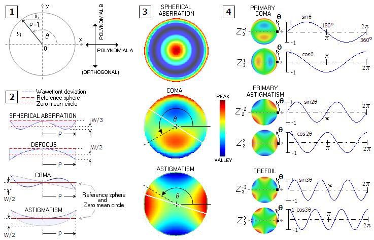
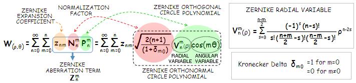
► 3.5.2. Zernike aberration polynomialsPAGE HIGHLIGHTS An alternative way of describing best focus telescope aberrations are Zernike circle polynomials. These polynomials, introduced by the Dutch scientist Fritz Zernike (Nobel prize laureate for the invention of phase-contrast microscope) in 1934, can be applied to describe mathematically 3-D wavefront deviation from what can be constructed as a plane - i.e. unit circle - of its zero mean, defined as a surface for which the sum of deviations on either side - opposite in sign one to another - equals zero. Each polynomial describes specific form of surface deviation; their combined sum can produce a large number of more complex surface shapes, that can be fit to specific forms of wavefront deviations (aberrations). In principle, by including sufficient number of Zernike polynomials (commonly referred to as terms), any wavefront deformation can be described to a desired degree of accuracy. The usual way of applying Zernike terms is to the specific wavefront shape, which is "decomposed" to a needed number of terms in order to determine: (1) the main forms of contributing deviations, and (2) the overall magnitude of deformation. For simple aberration forms, such as pure Siedel aberrations, a single polynomial suffices. Describing more complex aberrations, such as, for instance, seeing error, as well as wavefronts formed by actual (i.e. imperfect) surfaces, requires an expanded set of Zernike polynomials.
Zernike polynomials define
deviations
from
zero mean as a function of the radial point height ρ
in the unit-radius circle and its angular circle coordinate θ, which is the
setting of a telescope exit pupil,
in which the wavefront form is
evaluated (FIG. 30, 1). In
polar and Cartesian coordinates, respectively, the radial component is ρ2=x2
+y2,
with 0≤ρ,x,y≤1.
The common convention for the angular coordinate θ varies
with the field; in ophthalmology, it is
counterclockwise from x+ toward y+ axis (OSA recommended),
thus ρ=x/cosθ=y/sinθ. In general optics, it is often
different. Malacara's convention is clockwise from
y+ to x+ axis, thus ρ=x/sinθ=y/cosθ, and Mahajan's
convention (Optical imaging and aberrations) applied here to the conventional aberration functions is
counterclockwise from y+ to x-, hence with the same
radial-to-angular relations as Malacara's. The polynomials are orthogonal (i.e. their values change independently,
as illustrated on FIG. 30, 1) over the circle
of unit radius. Due to this
attribute, these aberration forms are termed orthogonal,
or Zernike aberrations.
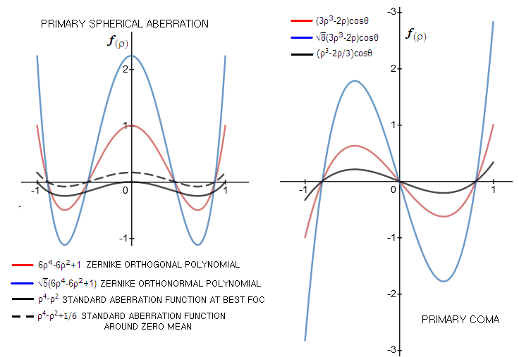
As mentioned, zero mean is defined as a surface for which the sum of wavefront deviations to either side is zero. That is important conceptual difference vs. standard wavefront error, which expresses deviations from a reference sphere (also commonly constructed as a circle). Hence the polynomial, which is a product of its radial variable in ρ and angular variable in θ, has zero value at the intersection of the wavefront and its zero mean. Zero mean differs from the reference sphere for balanced primary spherical aberration and defocus, while coinciding with it for balanced primary astigmatism. coma and balanced 6th/4th order spherical (FIG. A, 2). As a result, the form of polynomial is different from the classical aberration function for the former three, while identical (except for the normalization factor) for the latter two.
The polynomial normalization factor fulfils the formal requirement that
the radial polynomial portion equals 1 for
ρ=1. For instance, the deviation from zero mean for primary spherical
aberration - whose polynomial only has the radial component - is given
by ρ4-ρ2+1/6;
thus, its normalization factor is 6, and the corresponding Zernike
circle polynomial is 6ρ4-6ρ2+1
(this normalization to unit radius shouldn't be confused with
normalization to unit variance, described ahead).
Orthogonality of Zernike polynomials creates the possibility to combine
as many different surfaces as needed to approximate the form of
wavefront deviation with desired accuracy. It allows expressing separate
contributions of various forms of aberrations - including any chosen
extent of the higher order forms - and obtaining the combined variance
as the sum of individual aberration variances. Also, the polynomials can
be - and routinely are - scaled to unit variance over the circle radius
for all aberration forms, so that their combined form can be determined
directly by adding up their expansion coefficients, which determine the
specific magnitude for each aberration form. Wavefront is described
as a sum of Zernike aberration terms (FIG. 31).
In the nutshell, the normalization factor N is chosen so that a
product of the sum of two extreme values of the polynomial (absolute
values, determining the relative magnitude of P-V deviation) and
normalization factor equals the P-V-to-RMS wavefront error ratio for the
aberration. Hence, multiplying this product with the expansion
coefficient - which equals the RMS error for given aberration - yields
the P-V wavefront error corresponding to the coefficient. For any value
of the polynomial for given pupil coordinate ρ,
a product with the normalization factor and expansion coefficient
yields, as already mentioned, the wavefront deviation from zero mean for
that particular pupil coordinate.
EXAMPLE: Plots for orthogonal and orthonormal
Zernike polynomials vs. those of the standard aberration function for
primary spherical aberration and coma. All plots for either aberration
represent the same type of function - i.e. form of deviation - the only
difference being in their nominal maxima or position vs. abscissa
(horizontal scale), which represents the pupil, with the pupil radius
ρ normalized to unit ranging from -1
to 1. Function
f(ρ
)
- which is the wavefront deviation over pupil (with
θ=0 for coma) -
shows how the aberration changes over the pupil. In general, plots for
Zernike terms have significantly greater amplitude than the
corresponding standard functions, due to the coefficients (integer
multiplier assigned to the variable) being larger.
As with the standard aberrations, the wavefront error, either P-V (as a
direct optical path difference) or RMS, is directly related - although
not identical - to the phase error. The absolute value of
Zernike expansion coefficient
znm
is identical to the RMS wavefront error; since the coefficient does
express positive and negative deviations, the sum of coefficients for
all Zernike terms used to fit particular wavefront gives its overall RMS
wavefront error (i.e. standard deviation), and its square equals the wavefront
variance.
The two integers identifying Zernike aberration form
are n, the highest order (exponent) in the polynomial's radial variable V
(analog to the pupil height factor ρn
in the standard aberration functions)
and m, the angular frequency of meridional variance (nominally identical to
the exponent in the image height factor hm
in the standard aberration functions).
For radially symmetric aberrations,
like spherical, the angular variable
cos(mθ) or sin(mθ) is absent, thus m=0 (alternately, since it is
independent of the height h in the image
space, m=0); and, since the aberration changes with
ρ4
,
n=4. For primary coma, which changes with ρ3
and h, n=3 and m=1; since it varies
with the point pupil angle θ, it also includes the angular
coordinate factor, in the form cos(mθ).
Consequently, Zernike aberration terms for primary spherical aberration
and coma are denoted as Z
As mentioned, every Zernike aberration
term (or mode) describes specific orthogonal wavefront deviation
from its zero mean, that is, deviations from zero value of the
polynomial as a function of change in radial coordinate ρ
and angular coordinate θ. How Zernike
aberration term - i.e. orthonormal polynomial - specifically describes an aberrated wavefront is
illustrated on primary spherical aberration (FIG. 32). For
simplicity, the polynomial Z
Zernike
aberration term, either for the phase (Φ
S)
or wavefront (ZS,
identical to W(ρ)
,
the latter being used to relate the nature of it more directly)
deviation
for lower-order spherical is zero when the sum in brackets is zero. This
occurs for ρ2
=0.5±
1/√12,
regardless of the size of aberration, since the sum of
deviations between these two zonal heights is identical to the sum of
deviations over the rest of the wavefront (which are of opposite sign relative to the plane of
zero mean).
FIGURE 32: Zernike circle polynomials can be
used to express the two main aspects of wavefront aberrations: linear
deviations away from the reference sphere on one side, and closely
related to it phase error on the other. The former is described by the
wavefront aberration term Z
Here, linear wavefront deviation W(ρ)
,
specified by, and equal to the Zernike aberration term, is different
form the peak, or P-V value given by the standard aberration form,
because zero mean does not coincide with the reference sphere. However,
for aberrations where the two coincide - such as primary coma and
astigmatism - Zernike aberration term equals
the wavefront peak, or P-V error corresponding to the absolute value of Zernike
expansion coefficient, i.e. the wavefront RMS error (Zernike
coefficient, unlike RMS wavefront error, can be negative, since its sign
identifies the spatial orientation of deformation; the sign is determined by
the direction of wavefront deviation from reference sphere, along the
axis of aberration: if it adds to the OPL, coefficient is positive, and
vice versa - on the above illustration, for wavefront converging to the
left, the deviation adds to the OPL, and the sign of coefficient is
positive).
For instance, Zernike term for primary coma, Z
Likewise, Zernike term
for primary astigmatism Z
As another example, Zernike aberration term for
6th order
spherical aberration - the form that is optimally balanced with
4th order spherical - is given by the polynomial ZS
= √7(20ρ
6
-30ρ
4+12ρ
2
-1)z
S.
The zero mean is at the plane containing √0.5
zone (for pupil radius normalized to 1) - as well as two others for
which the polynomial is zero - on the wavefront deviation plot. The P-V
wavefront error is determined by a sum of the absolute values of
maximum deviations from the zero mean, which occur for ρ=0 and ρ=1.
With ZS
=W(ρ),
and z
S=ω
(the RMS wavefront error), this
gives the P-V wavefront error as W=2√7ω.
Since the P-V wavefront error for
lower-order spherical aberration, as already mentioned above, is a sum
of the deviations for ρ=1 or ρ=0,
and ρ=√0.5,
it is given by W=1.5√5ω,
and its P-V error for given (identical) RMS wavefront error relates to
that of the balanced 6th order aberration as
1.5√5/2√7.
Another interesting property of the Zernike aberration terms implicated by
FIG. 32 is that the P-V/RMS ratio can be expressed as (1+d)N,
where d is the maximum relative wavefront deviation from
zero mean (as an absolute value) to the side opposite to the reference
sphere - which is always in the plane containing the vertex - in units of the deviation from zero
mean toward reference sphere, and N is the term's
normalization (square root) factor. For most aberrations (all
primary aberrations except spherical, as well as all secondary
aberrations, including trefoil and spherical), |d|=1 and the P-V/RMS ratio
is given by 2N. So for coma, with the normalization factor equaling
√8,
the P-V/RMS ratio is 2√8,
and for astigmatism, with normalization factor
√6,
the P-V/RMS ratio is 2√6.
For primary spherical aberration, as shown on FIG.
32, |d|=0.5 and
the P-V/RMS=1.5N=1.5
√5.
As already mentioned, most common conic aberrations can be described
with a single Zernike aberration term, with either cosine or sine
angular function (the choice only affect wavefront orientation). However, in order to describe
wavefronts generated by
irregular surfaces - with this qualification applying to some
degree to all actual optical surfaces - or random aberrations (for instance, wavefront error
caused by atmospheric turbulence), multiple Zernike terms, with both
sine and cosine orientations, need to be included. Following page
presents in more detail the properties of Zernike aberrations for common
lower-order aberrations, as well as expanded list of Zernike terms -
often inappropriately referred to as "Zernike coefficients" - that
includes higher-order aberrations as well.
|