|
telescopeѲptics.net
▪
▪
▪
▪
▪▪▪▪
▪
▪
▪
▪
▪
▪
▪
▪
▪ CONTENTS ◄ 14.1. Early telescopes ▐ 14.3. Observatory telescopes ► 14.2. ATM TELESCOPES
•7" f/8 modified Sigler-Maksutov-Cassegrain
•30-inch f/5 Mersenne
Most ATM telescopes are of known designs, but their makers can customize
them to their liking. That makes them sort of unique, and adds to the
satisfaction of accomplishing, sometimes very challenging, creative
projects. With more complex systems, it all starts with a design created
and optimized through raytracing, as the basis for elements'
fabrication. And some of ATM telescopes are truly unique systems, out of
common knowledge of the amateurs and professionals-alike.
Marc Baril's 7" f/8 modified Sigler-Maksutov-CassegrainMaking Maksutov-Cassegrain of any kind is not for the faint of heart, primarily due to the full aperture Maksutov lens corrector, whose "easy" to make spherical surfaces have to remain within tight tolerances for the surface itself, the two surfaces relative to each other, and both relative to the meniscus thickness. A good example of it is Maksutov-Cassegrain made by Marc Baril, an amateur astronomer with professional background. Main modification to the Sigler's design was shortening the tube length which, according to Baril, did somewhat lower system's axial correction, but still allowed a high-level performance. Here is raytrace of the prescription given in the article.
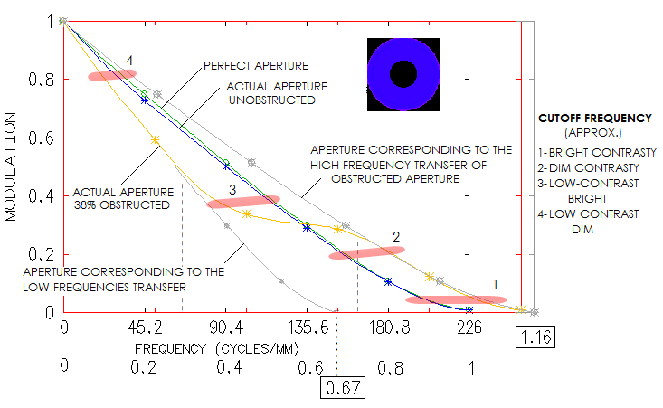
Design shows great field correction, with near-zero coma and astigmatism (it could, in fact, have 2-3 inches - or even more - smaller corrector separation without perceptibly affecting coma correction). Correction barely changes going from the field center to 0.5 degrees off axis. One thing to notice is that axial monochromatic correction of the starting design is a bit off (top left). It looks like undercorrection, but it is suboptimally balanced 6th/4th order spherical, with the lower order (undercorrection) being nearly twice larger than the (overcorrected) higher order. With the RMS wavefront error of 0.043, it is at the level of just a tad stronger than 1/7 wave P-V of lower order spherical. Baril mentions having a slight undercorection when arriving at the testing stage, which he removed by working the first corrector radius with a petal lap. While he thinks that what it did was slight aspherising, even just a slight strengthening of the first radius - going from 10.3507" to 10.344" - would do the trick. After taking care of undercorrection, we come to a design with 0.982 Strehl in the e-line, 0.927 in the F, and 0.926 in C. The polychromatic (430-670nm photopic) Strehl is 0.964. If we minimize the chromatism by bringing the colors tightly together strengthening corrector radii to 10.05" and 10.481", the two lines go to 0.972 and 0.976, respectively, with the e-line at 0.98. The polychromatic Strehl goes to 0.977. The Strehl figures are actually somewhat improved due to the 38% central obstruction, which took out the central deformation of the wavefront caused by spherical aberration. But the central obstruction did, of course, more damage than good at the level of system's PSF. Still, it's negative effect is commonly exaggerated. Baril states in his article that the biggest disadvantage of this design is its large central obstruction. How big a disadvantage it really is? The fact is that it reduces the wavefront error in all wavelengths - the larger wavefront error, the more so. If we would take it out, these same optical surfaces would produce wavefronts of lower quality. The central line, for instance, would go from 0.183 wave RMS and 0.982 Strehl, to 0.0225 wave RMS and 0.972 Strehl. At the same time, obstruction causes 0.86 drop in the relative central intensity of the diffraction pattern, with the second 0.86 reduction factor for the energy contained in central maxima - 0.73 reduction in total - coming from the reduced central maxima size. Due to the size reduction, central maxima is not only smaller, allowing higher limiting resolution, but also significantly brighter than what 0.73 degradation factor implies. In this case, central maxima is only 7% less bright than in a perfect aperture, in this respect corresponding to 0.93 degradation factor. So, while the nominal degradation factor is 0.74 (rounded from 0.73*0.982/0.972), it is also accompanied by 13% higher limiting resolution, and higher contrast transfer in the high frequency range. MTF compilation below illustrates the magnitude of both, loses and gains.
Here we see that the worst part of the central obstruction effect is lowering contrast transfer to the level of 33% smaller aperture in approximately 0-0.3 range of frequencies. In the 0.7-1 range the transfer increases to the level of 16% larger aperture, while over the 0.3-0.7 range we have transition from lower to higher transfer, extending all the way to the resolution limit of 16% larger aperture. Overall, nominal view favors obstructed aperture, which has contrast transfer advantage in nearly as much of the frequency range as the unobstructed, with extra high frequencies added beyond the resolution limit of unobstructed aperture. However, to better understand the implications, MTF frequencies should be associated with magnification. With the limiting resolution at cutoff frequency λ/D in radians (times 206,265 in arc seconds), magnification at which a general detail is magnified to 5 arc minutes (likely more near threshold of detection), needed for the average eye to recognize its shape is 300D/206,265λ, or 2.64D for the aperture diameter D in mm and λ=0.00055mm (67D for D in inches). For details of Airy disc size, 2.44λ/D, corresponding to 0.41 frequency, it is 1.1D, and half as much for twice larger detail (0.2 frequency). So we could say that high magnifications start, quite approximately, at 0.3 frequency. If so, the bad part of central obstruction effect falls to the range of mid and low magnifications, while the good part covers most of the high magnification range. That said, should be noted that the largest contrast drop for this obstruction, some 25%, is at about 0.4 frequency - somewhat deeper into the high magnification range - while diminishes toward the mid-to-low magnification range (<0.3 frequencies), down to 12% at 0.2, and 5% at 0.1 frequency. There are direct implications of different contrast levels on the limiting resolution. Taking approximate minimum contrast requirements for different object types from Rutten/Venrooij, we get that the obstructed aperture will have appreciably higher resolution limit not only for the conventional MTF limit (two bright lines, nearly identical to that for two near equally bright stars), but also for bright contrasty objects, like the surface of Moon (1 and 2, respectively). On the other hand, unobstructed aperture has higher resolution limit for bright low-contrast objects (3) and dim low-contrast objects (4). Obviously, we can't compare apples and oranges, so whether the effect of central obstruction is good, bad, or insignificant, will depend on the specific use. In all, the effect of central obstruction is a mixed bag, and certainly is not only bad. For photography, considerations are somewhat different, but the effect is generally considered less of a factor than for visual use. Summing it up, while it is not possible to execute the actual optics to its theoretical optimum, it is not even necessary. No mortal soul can see the difference of one or two 1/100s in the Strehl ratio. From Baril's article, it is very likely that his commitment to making this telescope as close to its design marks as he could, did bring it to the level where the difference vs. theoretical optimum didn't matter.
Sure, performance level would have been even better with a system with
slower primary, such as the original Aries' Maksutov Cassegrain, without
significant difference in the tube length. But if one wants a faster
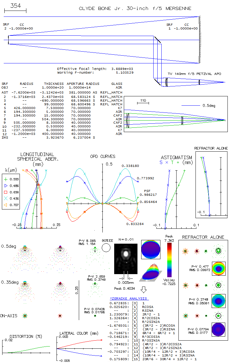
system, there is a price to pay. Clyde Bone Jr. 30-inch f/5 MersenneIn an S&T article from 1999 Clyde Bone (San Angelo, Texas) describes his 30-inch f/5 Mersenne-type telescope, for which he used Tele Vue's 140mm f/5 Petzval apo at the eye end (there is also an article on the Tele Vue site). The telescope was built with the highest standards, using, for instance, astro-Sital mirrors with 96% reflectivity - 1/16 wave primary, 1/10 wave secondary - and Pyrex flats with dielectric coatings (98.5% reflectivity). The two mirrors are confocal paraboloids, producing collimated beams free of aberrations (except Petzval image curvature, which is here -836mm). An image-forming system is required and, if the completed system is to be a visual telescope, it has to consist of an objective and eyepiece - i.e. telescope. Image below shows raytrace of such a system. Since no information on the Tele Vue refractor was published, a Petzval system that should be similar to it in its optical output is used to illustrate the combined performance level. It is a borderline "true apo" based on the errors in the four unoptimized wavelengths (F and C balance out at about 0.80 Strehl, and only the violet g-line is little over the required 1/2 wave P-V), but not according to its 0.917 polychromatic Strehl (photopic). This is mainly caused by keeping the violet g-line error nearly as low as possible, causing the blue and red - particularly the former - to be suboptimally corrected. If the F-line error is minimized, its Strehl increases to 0.856 (w/0.898 C-line), g-line drops to 0.183, but the poly-Strehl is up to 0.945 (all needed to accomplish this is to change R5 i.e. 9 in this prescriptionto 520mm, and R8 i.e. 11 to -237.7mm; that produces f/5.15 system, rescaling it to f/5 would lower the poly-Strehl to 0.934). The actual secondary is six inch in diameter, but in order to avoid stopping down the aperture, the reflected beam width has to be no more than 140mm (here, it is slightly less, which produces an effective f/5.1 system). Note that refractor alone is evaluated at f/5, and the setup used only stop at a distance of the Mersenne system exit pupil (located at -k+k2 from the secondary, toward primary's focus, in units of primary's focal length, with k being the marginal ray height of the axial pencil at the secondary, in units of aperture radius). Prescription with the complete system given with the image is a compilation of two prescriptions (OSLO Edu has 10-surface limit). This means that the nearly flat field here in the actual telescope corresponds (approximately) to the Petzval image surface, somewhat lessened by astigmatism induced by lens objective processing diverging pencils from the secondary (shown on astigmatism plots). Also, the 0.5° field radius in a 700mm f.l. refractor corresponds to 0.09° in the 3889mm f.l. system (will be explained ahead).
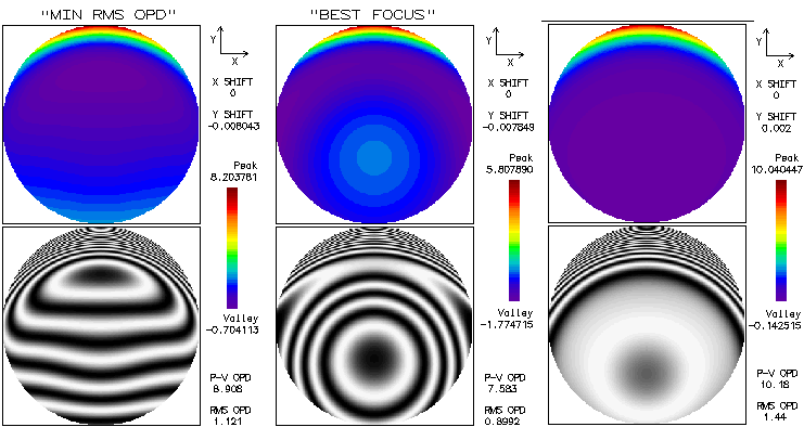
The field is limited to 0.5° i.e. 0.09° radius, since off-axis aberrations are already significant. It is a consequence of the widely separated aperture stop (also, as the box right from prescription shows, vignetting at the objective lens becomes significant). Part of it is that the incident ray angle is magnified after reflection from the secondary. With infinite secondary magnification, incident angle is magnified by a factor 1/k; with k=0.18 here, the incident angle magnification is 5.56, i.e. 1° angle at the primary becomes 5.56° at the lens objective. Hence, 0.5° at the lens objective is 0.09° in the actual system (linear field height is identical in both, since the two respective focal lengths differ by the same ratio). The central obstruction is 20% linearly, or little more. Since its effect on off-axis aberrations here is negligible, it is omitted to keep interferogram patterns intact. Also, to show the original polychromatic Strehl of the refractor, which would be superficially increased in the presence of obstruction (specifically, it would increase the poly-Strehl to 0.934 - and to over 0.95 with the F-line error minimized - as a result of small wavefront error decreases in all wavelengths - the larger error, the more - hence only in part reflecting better chromatic correction; on the other hand, that small gain is paid for with a 0.96 drop in central intensity - to the actual 0.897 - plus another 0.96 ratio energy loss due to the smaller central maxima, for the final 0.87 central maxima energy ratio on axis). Wavefont map for the 0.5° point shows that most of the P-V error comes from raised edge on one side. Because of that, both P-V and RMS error are somewhat misleading, implying larger than the actual error. The main wavefront component is in the blue area, less than 1/3 of the entire 8 wave P-V error. Zernike analysis gives as dominant terms primary coma (#6), astigmatism (#4) and defocus (#3), followed by secondary astigmatism (#11), coma (#13), primary spherical aberration (#8) and trefoil (#9). However, the primary spherical aberration term indicates 0.32 wave RMS, much more than what is present on axis; this means that most of this term is actually lateral spherical aberration, a secondary Schwartzschild aberration of the same form as primary spherical, but increasing with the square of field height. Also, raytrace shows that coma-like ray spot plot grows significantly faster than in proportion to field radius, indicating presence of other "odd" secondary aberrations, such as lateral coma (secondary Schwatzschild aberration, of the same form as primary coma, but increasing with the cube of field radius), and probably some others. Diffraction simulation for the 0.5° point (e-line) shows some elongation, but still well formed central maxima, embeded in a tight, bright ring (mostly due to 0.01 normalization); however, 80% energy radius is 0.0286mm (large black circle), much larger than the Airy disc (not sure how adequate is this number, since it could be based on PSF centroid location, which is here by some four Airy disc diameters - or 0.025mm - from the PSF peak, indicated by the dense ray area above the Airy disc circle on the ray spot plot). The bright central oval is similar in area to the Airy disc, but the peak intensity is only 0.40, indicating energy comparable to that with 1/2 wave P-V of spherical aberration (note that the peak intensity is much higher than central intensity, due to intensity shift from the PSF center). Box bottom right shows corresponding ray spot plots for the refractor alone, for the same 0.5° radius field; evidently, all off axis aberrations are a consequence of the large stop separation. There is a discrepancy between the 0.5° wavefront error magnitude and the corresponding PSF. Even if limited to the blue area on the wavefront map, it is as much as 2-3 waves P-V, not agreeing with still quite compact central maxima. Taking a closer look, we see that OSLO default wavefront map is for "minimum RMS OPD" (image below, left).
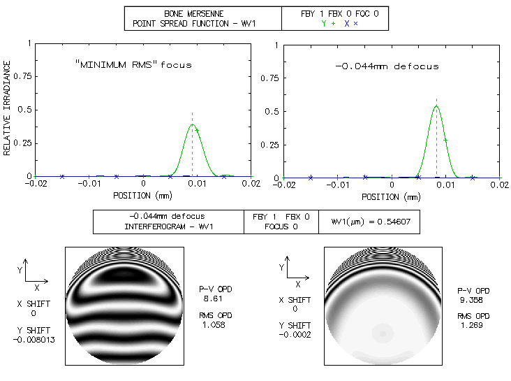
The corresponding interferogram shows that most of the blue area is tilted, with a small depression going into the raised upper edge. With the fringe-to-fringe separation being 1/2 wave OPD (optical path difference), the tilt of the blue area is little over two waves. Since tilt itself doesn't degrade point image, merely moves it in the direction of tilt, all needed to find the wavefront corresponding to the best image is to center it on that point (the raised edge adds another 5-6 waves, but it cannot be optimized tilt-wise simultaneously with the remaining, larger portion of the wavefront; its energy is, therefore, widely spread, contributing very little to the central diffraction maxima). The second OSLO option, "best focus" displays wavefront that combines tilt with a significant defocus over the blue area (middle). It actually has lower both, P-V and RMS error, with only a slight difference in the vertical shift (Y; the defocus shift along Z axis is not shown). In order to correct for the tilt alone, the third option, "reference ray intersection" needs to be used. Entering 0.002 Y-shift to the default coordinates, brings out the wavefront shape over the blue area for the best image proximity (right). It shows that most of this area is a low-aberration region, outlining a two-circle-intersection shape, oriented horizontally (the nominally higher overall P-V and RMS are the consequence of a larger error in the raised area, which is of little importance since it was already mostly wasted with respect to its energy contribution). This explains both, vertical elongation of the PSF central maxima and its integrity. Unfortunately, OSLO Edu has no option to calibrate PSF output with other than default data (it produces the best diffraction image decentered, in the process of generating PSF simulation for a wider area). However, entering -0.044mm defocus produces interferogram similar to that on the left, only with somewhat less of tilt in the blue area. For this point, PSF peaks at 0.52, suggesting it is the best focus (image below). Note that the actual PSF peaks are lower by 0.96 factor, or little more, due to the effect of central obstruction.
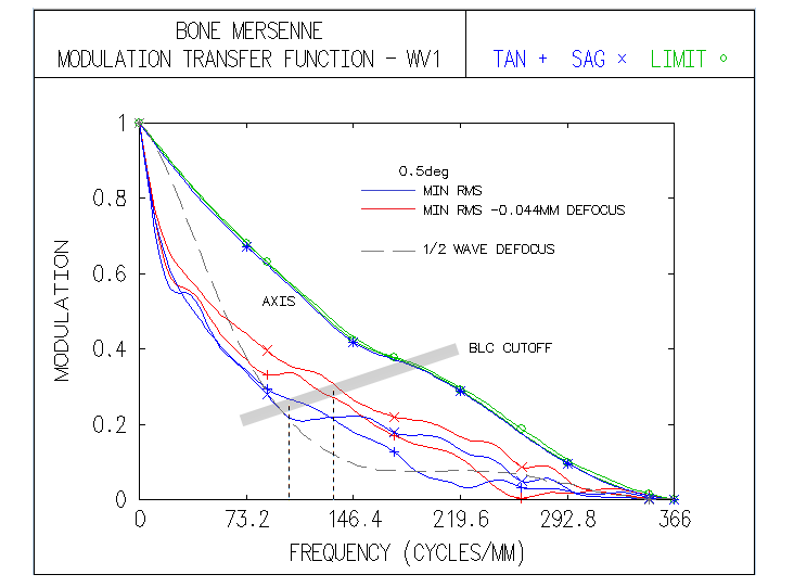
Note that even with OSLO making vertical shift adjustment, it is not the wavefront centered on the PSF peak, since it was looking for the "minimum RMS" error, and found it at an image point with still significant tilt error in the main, lower portion of the wavefront. If we manually enter -0.0002 shift - which should be equivalent of +0.0078 shift with respect to the default - we see interferogram nearly corrected for tilt and other aberrations (except a roughly 1/4 wave zone) in an area somewhat larger than with the "minimum RMS" focus corrected for tilt, which should be the reason for the higher PSF peak. But the P-V and RMS wavefront error are again larger for this point. This illustrates why both, nominal P-V and RMS wavefront error become less reliable indicators at large error levels. The "best focus" option is supposed to find what it promises, but it evidently doesn't always work as planned. Contrast transfer plots below show the defocused image at 0.5° as having appreciable higher contrast transfer than the "minimum RMS" focus. Note that these plots do include the effect of 20% linear central obstruction, omitted above.
The contrast advantage results in a significantly better limiting resolution of the defocused "minimum RMS" image for bright low-contrast (BLC) details. For comparison, dashed plot shows contrast transfer for 1/2 wave of defocus (unobstructed aperture). Tolerance to miscollimation between the mirror and telescope axis is comfortable: 5mm decenter will lower the central e-line Strehl to just below 0.95, while 0.5° tilt at the objective - implying 4.4mm axis-to-axis deviation 0.5m behind - lowers the Strehl to 0.96. However, 1° tilt already induces over 0.4 wave P-V of all-field (even magnitude across entire image) astigmatism, with the Strehl dropping to 0.73. Miscollimated secondary would induce combination of tilt and decenter. Considering large separation, it is the most sensitive part of the system. As little as 0.1° of tilt would translate to 5.5mm decenter combined with 0.2° tilt.
Replacing the above Petzval refractor with two others (FPL53/ZKN7 and
FPL53/BK7; the former has 0.999 central line Strehl, similar error magnitude in the g-line,
but tighter rest of them, resulting in 0.954 polychromatic Strehl,
while the latter has the central line Strehl already below 0.95,
due to more of higher order spherical residual), all with different
limits to spherical aberration correction
show that off axis aberrations in this setup mainly result from
uncorrected spherical aberration in the refractor: the more of it, the
larger off axis aberrations induced (uncorrected off axis aberrations
also are a
factor when present). Since in this demonstration the refractor limit is at
0.018 wave RMS, or less than 1/16 wave of primary spherical, the actual units
would produce more of off axis aberrations, and significantly so. For instance,
the FPL53/ZKN7 combination has only 2.4 wave P-V wavefront error of
the same form at 0.5°, and we are talking 1/51 vs. 1/16 wave P-V
of primary spherical aberration (the FPL53/BK7 combination, with 1/8 wave
P-V of primary spherical equivalent, has as many as 22.3 waves P-V
at 0.5°). Considering
that this field size (0.18° diameter in the actual telescope) is
already within its medium-high magnification range, there is no room to absorb further field
definition worsening. It is wise not to push too far with the
objective speed: all else equal,
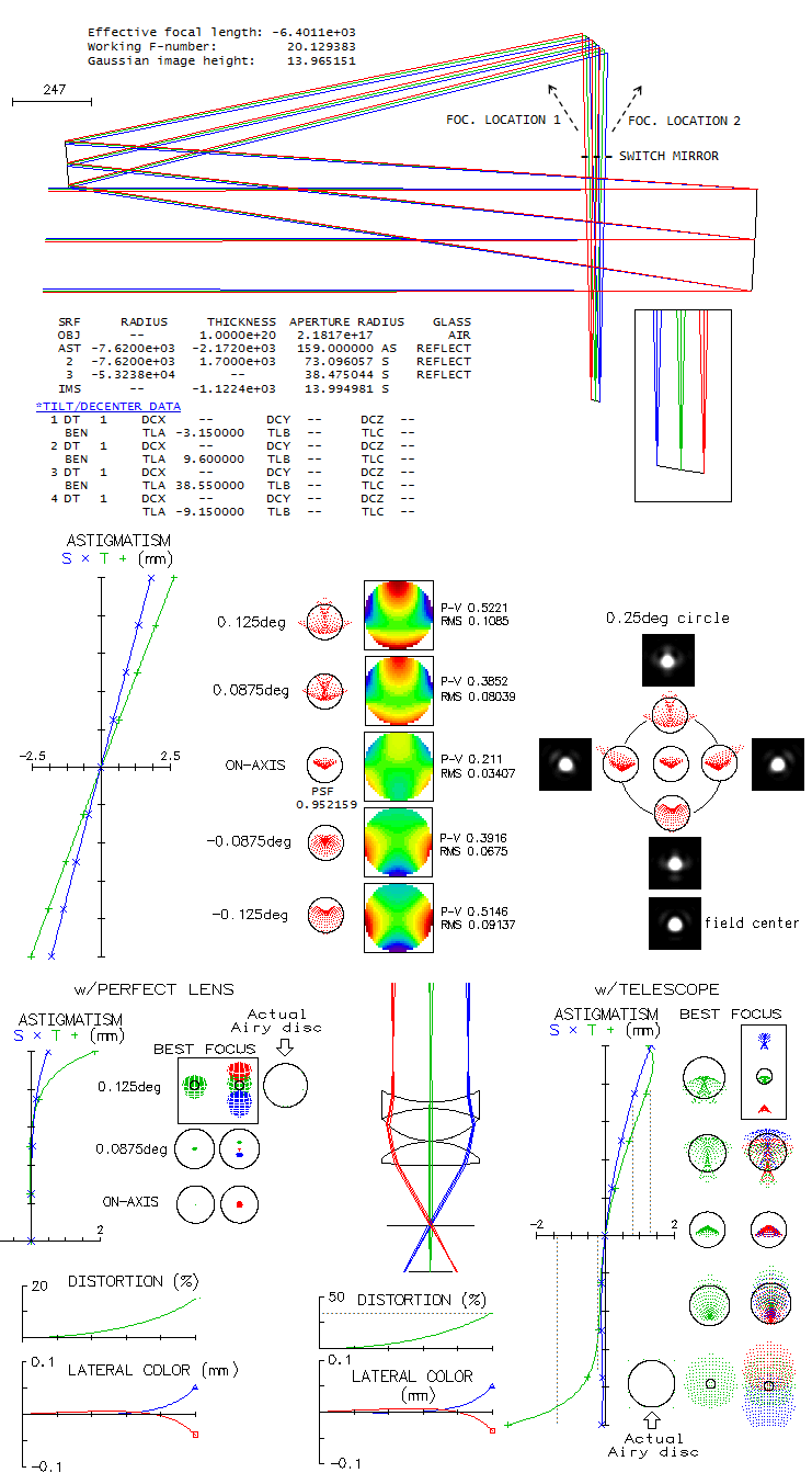
an f/6, or f/6.5 could do noticeably better in this respect than f/5. Terry Platt's 318mm f/21 Buchroeder "Quad-Schiefspiegler"Described in detail in Tonkin's "Amateur Telescope Making", this tilted-mirror system stems directly from Kutter's Schiefspiegler, with the third mirror added to cancel out astigmatism once the primary and secondary are arranged to cancel out coma (in the book it is called "quad-schiefspiegler" but since reflecting flat does not influence system output, it is a three-schiefspiegler). Reflecting flat is added in order to create two alternative focus locations, as indicated below. However, since it doesn't influence raytracing, and the telescope is fully operational without it, it was omitted from consideration. Primary mirror is aspherized (-0.55 conic) in order to minimize axial aberration, with spherical secondary and tertiary. Field angle is chosen to create image that fills out 1.25-inch barrel.
Astigmatism plot reveals significant image tilt. At the field edge, defocus due to the tilt is over 2mm, or over 1 wave P-V. However, what matters is how much of accommodation it will require in the image formed by the eyepiece. Axial correction is much better than in the Schiefspiegler (considering three times larger aperture), with the design limit better than 0.95 Strehl. According to Zernike wavefront decomposition, nearly 90% of the axial aberration is trefoil, with some residual coma. Longitudinal astigmatism of 0.85mm at the top edge (somewhat less at the bottom) implies 0.44 wave P-V wavefront error of astigmatism, which makes it dominant aberration in the outer field, with small contributions from trefoil and coma. Field aberration is not radially symmetrical, but it is relatively insignificant since at the very edge of the field central diffraction disc remains well defined. The maker of this telescope states that the image tilt - which is over 9° - does not significantly affect observing. It shouldn't be a surprise, considering the slow f-ratio, but it can be informative to assess it specifically with raytracing. Using 30mm f.l. 2+1 Koenig design, ray spot plots are shown for a perfect telescope (bottom left) and the actual telescope (bottom right). Note that the field angle is too large for this particular eyepiece design, requiring lenses larger than 1.25 inch barrel, and resulting in a sharp increase in the field edge aberrations (the corresponding undistorted field of view is over 53 degrees which, with 15% positive distortions produces 61° AFOV; a bit too much for a 50° AFOV design). Except the perifferal field, telescope aberrations dominate, which was to expect with this slow f-ratio. The effect of image tilt only shows toward field edge, increasing eyepiece aberrations on the bottom, and decreasing them on the top (the two field sides should have edge astigmatism at the level of the eyepiece in a perfect system). Accommodation required for the field edge is less than 1.5mm which, for 30mm f.l. eyepiece i.e. diopter equaling 0.9mm, translates to nearly 1.5 diopter of accommodation (infinity to 0.67m), positive on the field top, negative on the bottom. Without excessive edge astigmatism of the eyepiece, accommodation required would have been yet smaller.
In all raytrace confirms that the telescope, as a design, offers
well corrected field despite nominally significant image tilt.
That, however, assumes well collimated system. The 0.80 axial Strehl
tolerance for tilt is 0.025° (less than 1/14mm deviation
at the edge) for the primary, 0.05° for the
secondary, and 0.035° for the tertiary (for the aberration
induced by tilt added to the existing design minimum). Since this is
with the "tilt and bend" choice "on" - meaning that change in tilt
of the primary automatically adjusts axial position of the
secondary and tertiary (and change in the secondary's tilt adjusts
position of the tertiary) - the actual tilt tolerances should be
tighter. On the other hand, secondary and tertiary
are relatively insensitive to decenter (up to a few mm still leaves
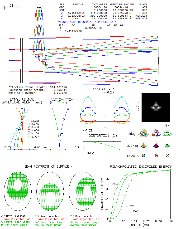
the Strehl well above 0.80). Bratislav Churchich's 146mm f/3.9 Wright cameraMuch less well known than its older cousin Schmidt camera, the Wright camera is not as well corrected, but has features that can make it preferred choice for some applications. In relatively slow systems, correction difference becomes less important, and its better compactness and inherently flat field can overcome the disadvantage of having to make an oblate ellipsoid for the primary and twice stronger Schmidt-type corrector. The latter apparently wasn't an obstacle for Churchich, who in order to make the camera more compact decided to go with even more strongly aspherized primary (nearly 1.5 conic), which also required as much stronger Schmidt corrector. As he describes in the same Tonkin's book, he stopped a bit short of the optimum primary conic (1.5) preferring to keep an exceptionally smooth figure. All this makes his Wright camera different from the standard. The corrector was made with 70.7% neutral zone, being the easiest shape to fabricate, but it also has the lowest spherochromatism (86.6% neutral zone has the smallest blur, but over 2.5 times larger wavefront error). Table below describes the perfect Schmidt profile needed for this instrument. Any deviation from it generates wavefront error by a 0.517 ratio (e-line), since the light speed in the BK7 glass vs. air is 1/1.517:1.
It shows that its maximum depth is less than 10 waves of 550nm light, i.e. that corrects mirror wavefront error 1.517 times smaller, around 6 waves P-V. The diagonal mirror is 55mm in diameter, taken as the size of central obstruction. Raytrace of this system below assumes perfect surfaces.
Due to the relatively slow focal ratio, chromatic correction is excellent, comfortably within the "true apo" requirements. The ray spot plots show residual coma (about 0.80 Strehl large at 1° off), but it is low enough not to significantly alter the shape of diffraction image (for fully canceling coma, either primary conic of 1.5, or corrector separation of 460mm are needed). The diagonal is not quite large enough to fully illuminate 2° field (it is raytraced w/o offset, but in the actual telescope is offsetted to be centered under the focuser). At the field edge, vignetting is about 10% (taken as that on the horizontal ends of the diagonal, the 3rd from left), which is within acceptable. Note that 711 out of 917 rays is what remains after central obscuration.
Since the main purpose of the instrument is imaging, what really
matters is size of the circle of energy. In this case, the camera
places 80% of energy into 8-micron circle on axis, 10-micron
circle at 0.7° and 14.8-micron circle at 1°. Angularly,
it corresponds to 2.9, 3.6 and 5.4 arc seconds. The actual star
image, as the diffraction images implies, is a bit larger, some
17 microns 1° off (of course, before seeing-caused bloating). The
Airy disc for an f/3.9 system is 5.2 microns in green light (546nm)
but these numbers are for the five wavelength from 436nm to 706nm
with even sensitivity. Since neither photo emulsion nor CCD have
flat sensitivity in that range, the actual circle sizes are somewhat
smaller. In this case, they were smaller than the typical photographic
blur, despite the unplanned, not negligible spherical aberration
residual. If the system was built as the standard Wright, with
a weaker primary and corrector, the 80% energy circle 1° off
axis would have been 13 microns, not much smaller than 14.8
microns in Churchich's customized camera (if optimized by
going for 1.5 primary conic,
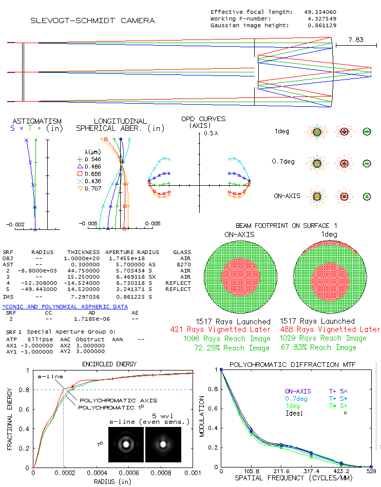
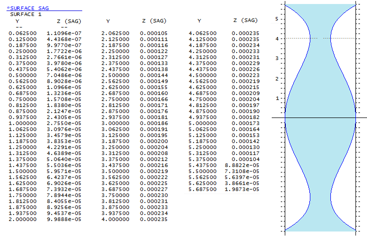
the circle would measure 13.6 microns). Dan Cassaro's 11.4-inch f/4.3 Slevogt-Schmidt cameraAlthough still in making, this ATM camera posted at the CloudyNights forum is both, interesting and challenging. In order to obtain flat field with the Schmidt corrector and two spherical mirrors, corrector needs to be widely separated from the mirrors. The alternative is the Write-Schmidt, less than half as long, but with significantly more field astigmatism, and requiring a hard to make oblate ellipsoid as the main mirror. Its advantage is significantly smaller central obstruction, but if field quality is main concern, Slevogt-Schmidt is the way to go.
Design data posted at the forum describe a 11.4-inch f/4.33
Slevogt-Schmidt with f/2.294 spherical primary. It implies
secondary magnification of 1.89 which, for given back focus
distance, supplies necessary data to calculate the rest of
needed parameters: mirror separation, i.e. hight of the
marginal ray of the axial beam at the secondary, secondary
radius of curvature, corrector separation and aspheric
coefficients (mirror and corrector separations are already
given with the system, as well as secondary radius of curvature,
but the design usually starts with the primary, final f-ratio
and back focal length as the basis for calculating remaining
parameters). In general, in order to have flat field
Slevogt-Schmidt needs to have secondary radius of curvature
about 0.96 of the primary's, and secondary magnification about
1.8. Denoting needed parameters as
Raytrace shows excellent color correction, with as litle as 0.26/0.06
P-V/RMS wavefront error in the violet g-line. Astigmatism is very low,
reaching 0.22/0.05 P-V/RMS error 1° off axis on flat field;
central diffraction maxima is well defined all the way to the field edge. To
fully cover the 2° field the secondary would have to be 6.48 inch
in diameter, or 57% of the aperture diameter clear area only. Somewhat
smaller secondary would be acceptable: shown is vignetting with the
secondary clear area 6 inch in diameter: it is still only 6.1% at
1° off axis (circular red area is vignetting by the central
obstruction). Considering that the reduced central obstruction
would recover nearly 5% of light over entire field, including
edge, field illumination actually improved with smaller secondary.
Both, encircled energy plot and MTF show near-negligible drop to
the very edge of the field (note that polychromatic refers
to the five wavelengths plotted, for even sensitivity; it indicates
that the actual CCD performance is little better).
While given prescription indicates neutral zone near 0.707 radius
height, which generates over two times smaller wavefront error
than neutral zone at the 0.866 height, raytrace show that the latter
would have actually a slightly smaller 80% encircled energy radius.
This is due to the effect of large central obstruction, reshaping
the wavefront to practically cancel much larger error.
Still, the 0.707 neutral zone corrector is significantly easier
to make: its maximum depth at the neutral zone is 2.25 times smaller.
Note that the actual corrector here is with split profile, i.e.
each side gets half of it, but the effect is the same as with a
single side profile. Table below shows surface profile as the sag
values at each 1/16 inch of aperture radius. At right is exaggerated
profile with a quarter inch scale.
Would the image quality be better going with ρ=0.96 and m=1.8?
It would result in somewhat smaller secondary, but the back f.l.
would be reduced to 5 inch, with the RMS WFE 1° off axis
slightly higher. Extending back f.l. to 7.2 inches by placing
secondary closer to primary would change the value of k
and make best image surface slightly convex toward mirrors (R~2500),
only slightly worsening the RMS WFE 1° off axis (0.055 vs. 0.054).
Extending back f.l. by strengthening the secondary radius would
make best image surface concave toward mirrors (R=-166), with
the error 1° off axis cut in half on the best surface, but
increased to 0.15 wave RMS flat. Hence, when significantly
changing back f.l. determined by m~1.8 and ρ~0.96, using
equality m=ρ/(ρ-k), balk of the change in secondary
magnification should come from the change (increase for extending
back f.l.) in k, with the change in ρ only
needed to offset the induced field curvature. In other words, to make
β=(m+1)k-1 by 46% longer (7.3 vs. 5 inch), most of the
increase is to be contributed by a change in k.
Looking at the astigmatism aberration coefficient for flat
astigmatic field and using starting values ρ~0.96, m~1.8,
a simple relationship approximating the needed change in ρ
to compensate for the change in k is ρ'=0.99-0.07k'.
In this particular case, k changes from 0.425 to 0.444,
and ρ from 0.96 to 0.956 (minor adjustments to the
aspheric coefficients and radius term are also needed).
The above raytrace is design limit; the actual output will be
negatively affected by alignment errors and thermal imbalances.
Tolerance for the corector-to-primary separation is fairly
loose, with the error due to coma at 1° off axis increasing
from 0.05 to ~0.07 wave RMS with about an inch off (little more
away from, little less than inch toward primary). Error of 0.1" in
mirror separation induces ~0.2 wave P-V of spherical aberration.
Secondary decenter of 0.1mm up induces over one wave P-V of mainly
positive all-field coma, with that error more than doubling at 1° off
due to the image tilt. Secondary tilt of 0.1° counterclockwise
(top away from the primary) induces nearly
one wave P-V of negative all-field coma, along with somewhat more
than half as much of image tilt as the decenter. Since the secondary is spherical,
there is an offsetting combination of tilt and decenter; in this case,
offsetting tilt for the 0.1mm decenter is 0.116°, but the error
1° off axis would double due to the residual image tilt.
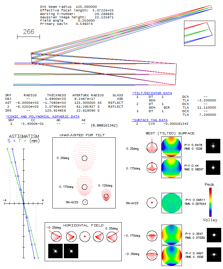
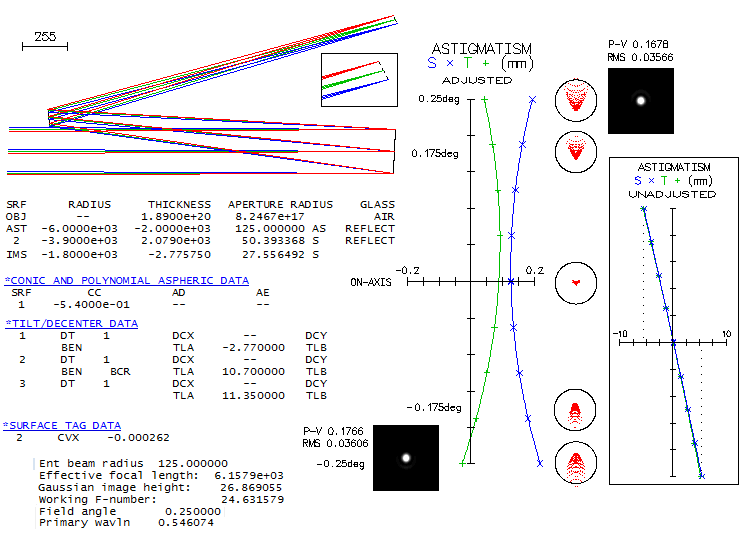
Built around 1998. this telescope of a renowned in ATM circles Dutch telescope
maker Rik Ter Horst, is a classical Kutter two-mirror tilted-components-telescope
(TCT) that instead of spherical uses toroidal secondary. It makes easier to
control aberrations of the two tilted mirrors, with the toroidal component
inducing mainly astigmatism. The system, as published on the Cloudy Nights
forum, consists of an ellipsoidal primary, little over half way between
a sphere
and paraboloid, and a toroidal secondary (below; if the primary is
left spherical,
the centerfield error is 0.022 wave RMS, mainly undercorrection, and if
paraboloidal 0.020 wave RMS of mainly overcorrection).
While Ter Horst describes sstem as free of coma and astigmatism,
it applies only to the
central field. Farther off, they are both present, with astigmatism
dominating. The
field of 0.25° is significantly larger than the intended field, as
indicated by the secondary cutting into the off axis light reflected from
the primary,
but it is chosen to illustrate correction over full 2-inch barrel field.
The intended
field is probably somewhat smaller than the 0.7 radius field here,
closer to half the
radius shown (about 1/4-degree in diameter). The astigmatism plot shows
the field edge
focusing nearly 3mm closer/farther than the central point (field top
and bottom,
respectively, mainly due to image tilt).
If this image is looked at with naked eye, from the least distance of
distinct vision
of ~25cm, the 3mm displacement of the top and bottom field point
amounts to little over 1/100
of the distance change, causing practically identical relative change
in the eye image location.
Assuming 17mm effective focal length of the eye, the top and bottom point
will be imaged
~0.17mm closer, i.e. farther away than the central point. In diopters,
the change amounts
to 1/0.01683 and 1/0.01717 vs. 1/0.017 for the central point, i.e. 59.42
and 58.24 vs.
58.82 for the central point, for about +/- 0.6 diopters accommodation.
For all practical
purposes, it is as good as flat.
Over best image surface, ray spot plots vary somewhat in shape with
radial orientation,
but diffraction images remain fairly similar for any given off axis d
istance, with the
central maxima remaining intact to the very edge. For the intended field,
even the very edge
is better than the "diffraction limited" minimum (0.80 Strehl).
Image tilt creates asymmetrical ray geometry with respect to the
eyepiece, hence always have
an effect on its output. As before, it is significant mainly toward top
and bottom of the field.
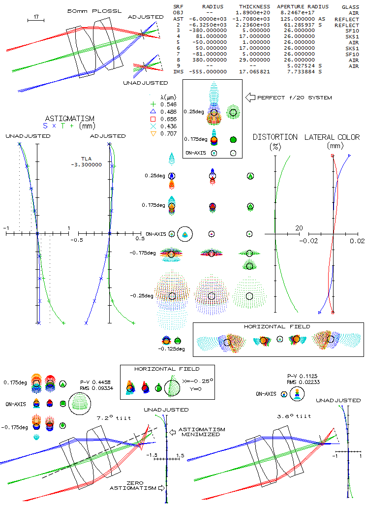
Taking again a 50mm Plossl (scaled down version of the patented Nagler
Plossl) to cover
the entire 2-inch barrel field, with a 17mm f.l. OSLO
"perfect lens" simulating the eye, the entire picture is scaled down as
it is in the eye,
with the image still tilted, but with somewhat modified, asymmetric
astigmatic field
(due to the asymmetric position of the eyepiece vs. image), creating
field curvature
element. Since the imaging element here is the eye, with 17mm effective
focal length,
one diopter of accommodation corresponds to 0.29mm point displacement
(from f2,
f being the f.l.). With the largest point displacement here of
about 0.6mm for
the top field point,
required accommodation is about two diopters, i.e. the visual field is
within easy accommodation
(since the top point requires extending converging beam, and the
bottom shortening,
they cannot be focused at at the same time, and the latter, requiring
lens contraction
is easier to the eye).
Note that it is important for the final image separation from "perfect
lens" to be
17mm, because it is its designated focal length, hence this image
separation indicates
that light pencils exiting eyepiece are collimated, i.e. that the e
yepiece is properly
focused; even small deviations, a few 10ths of
a millimeter from 17mm image distance represent change in ray geometry
that can result
in significantly different eyepiece aberrations.
Even when adjusted for tilt and field curvature, vertical field remains
very
asymmetrical, with mainly low residual coma on the top, vs.
significant astigmatism on
the bottom. Again, the diference diminishes significantly over the
intended field, about
twice smaller. The common wisdom is that the definition improves with
tilting eyepiece
to match image tilt (7.2° here), but things are not that simple.
Tilting the eyepiece
to match image tilt makes it asymmetrically positioned vs. optical axis,
and that also
have negative consequences. In this case, it greatly reduces astigmatism
over entire
field, except the top portion (not within the intended field area), but
at the same
time induces significant astigmatism (and a bit of coma) to the axial
cone, which is now
shifted somewhat below
geometrical field center (bottom left, dashed line crossing). Exit
pupil is also shifted significantly
below eyepiece axis, and is grossly distorted ("perfect lens" modifies
cone geometry
in order to remain aberration-free, but the actual eye does not have
that ability,
and would likely induce additional aberrations due to the exit pupil
disarray). Half as
much tilt of the eyepiece does better overall job, reducing the bottom
field astigmatism, with
about four times smaller error induced to the axial beam, and
significantly smaller
exit pupil disarray (bottom right).
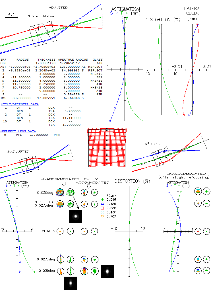
Going to shorter focal length eyepieces, for high magnifications, a
10mm Abbe orthoscopic with
~40° AFOV, when adjusted for image tilt and curvature (top)
shows asymmetrical vertical field,
with significantl more of astigmatism toward field bottom. OSLO shows
grossly asymmetrical
distortion as well, but it could be an artefact of field rotation.
Lateral color is nearly
identical on both sides.
Here, the maximal point displacement from the plane determined by the
central point is about 1.5mm (bottom left), which translates to 5.2
diopters of accommodation -
pushing the limit for the average eye. The main displacement factor
is image tilt, amounting to 13 degrees.
However, due to the tiny f/20 cones, even fully unaccommodated image
is still well defined
even at the field top/bottom (0.088 and 0.079 wave RMS, respectively).
Still, tilting eyepiece
to compensate for image tilt here further improves definition; a 6°
tilt nearly evens up the
astigmatic field, removing tilt element. Exit pupil is somewhat
decentered, but the axial cone
still nearly coincides with the field center. Longitudinal
astigmatism generated in the field
center is nearly 0.4mm, but due to the tiny cone width - effectively
~f/35 in the perfect lens,
from the eyepiece exit pupil diameter 0.49mm and 17mm lens focal length -
it converts to only 1/15 wave P-V.
A few general notes about the design. This particular system uses
secondary mirror somewhat
weaker than primary, probably to optimize the overall geometry for
desired setup. Stronger
secondary would make the final image separation larger, hence it would
need to be pulled
farther away from the primary, which in turn would enable use of
larger unobstructed fields.
Stronger secondary, in general, generates more astigmatism which,
being of opposite sign
of that generated by primary, results in a lower system astigmatism,
and with the optimum
match the astigmatism can be practically eliminated, leaving only a
slight residual coma (below).
The field is symmetrical, with the edge coma below the level of 1/8
wave P-V of spherical
aberration. The system is somewhat slower at f/24.6, due to the
larger primary-to-secondary
separation, but the overall length is comparable. One negative of
minimizing astigmatism is
nearly 50% larger image tilt, despite reduced tilt of both, primary
and secondary. This is
partly compensated by the slower f-ratio. There is any intermediate
combination of these
factors between the Rik Ter Horst's desing and this one, with
gradually diminishing
astigmatism, increasing image tilt and focal ratio reduction. As
indicated in the beginning,
designing with toroidal secondary is fairly easy. Since the final
field is in effect superposition
of two aberrated fields, those of the primary and the secondary,
partly compensating their aberrations,
appearance of center-field coma means that one of the two mirrors
has relatively stronger
tilt than the other. Assuming that the primary tilt is given,
positive center-field coma
indicates that the primary tilt is stronger than what it should be
relative to that of the
secondary (inducing coma of
opposite sign) for cancelled center field coma, and it is simple
matter of increasing
the secondary tilt until the center
field coma vanishes. Then center-field astigmatism can be brought
to zero by adjucting the
toric value (with the toric in OSLO nomenclature given as the inverse
of the toric radius),
which induces no appreciable coma. In the case of negative center
field coma, secondary tilt
needs to be decreased.
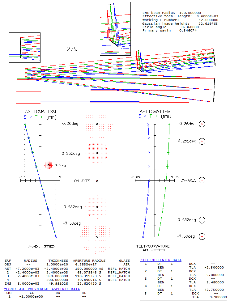
A work still in progress (as reported on the CloudyNights forum),
this big aperture tilted
element telescope consists of the paraboloidal primary, convex
spherical secondary and
concave spherical tertiary - the latter two of identical radius of
curvature - with a flat
mirror added to make the final image accessible. The actual system
may not be identical to
the published prescription, but differences should be negligible.
System shown below is
raytraced for the full 2" eyepiece barrel field, in order to
illustrate correction over full
field, but the actual design has field radius
limited to ~0.1° in order to minimize image tilt by keeping
mirror tilt to a minimum
(field can be significantly larger
if a small and generally negligible grazing of the axial cone by
the secondary is accepted).
Even with doing everything to minimize image tilt, it is still fairly
hefty, at 9.9°
(toward the end, the system variant covering the full field without
mirror obstruction,
with over 50% larger image tilt, will be analyzed).
Astigmatic plot for unadjusted field shows that the edge point
displacement is 4.2mm for full
field, and 0.9mm for 0.1° field. If looked by naked eye from ~25cm,
it represents 1.7% and
0.36% change in object distance vs. central point (respectively),
hence will induce practically
identical change in the point image separation in the eye.
In other words, the top full field point, being
farther away, will focus 1.7% of 17mm eye focal length closer, and
the top full field point, being
closer, as much farther away. In diopters, it is (1/0.017)*0.017=1,
which is practically as good as
flat. The field adjusted for tilt and mild curvature shows correction
far beyond the treshold of undetectable
across entire field. Through an eyepiece, however, both eyepiece
native aberrations and those caused
by the assymmetrically positioned field will significantly worsen
correction level.
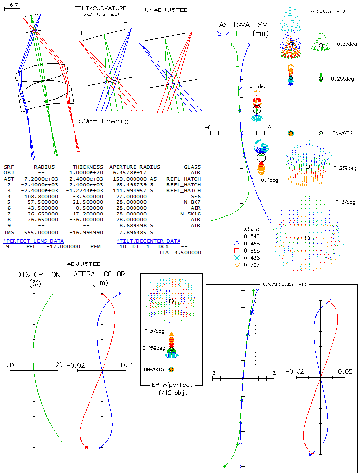
Starting with the full field, the corresponding conventional eyepiece
would be of ~50mm focal length.
Taking Koenig 2+1, comparable in its correction level to Abbe and
Plossl designs, shows that the
eyepiece image (it is actually image by the eye, in this case
simulated by OSLO "perfect lens",
of more or less collimated light pencils exiting eyepiece), expectedly,
suffers from significant
astigmatism assymmetry along the vertical field diameter. Top
astigmatic plot shows field adjusted
for tilt and relatively weak field curvature, so that the top and
bottom field point are near their
best focus. Since the astigmatism is a mixed lower and higher order,
in addition to the imbalance, field
curvature is irregular and most of the rest of the field along its
vertical diameter is not near its
best focus. However, the largest displacement from best focus is
about 0.2mm (less than 0.7 diopters,
with one diopter with 17mm focal length being
~172/1000=0.29mm; alternately, 0.2/17 times 59
diopters for the effective eye focal length in diopters). In other words,
when the adjusted field is
within the range of accommodation, the eye can see all its points at
their best focus.
As mentioned, field curvature element is relatively
mild, and needed corrective tilt is 4.5 degrees. In the unadjusted
field - the one that the eye actually
sees - it causes little over 0.8mm top point displacement,
and somewhat less for the bottom point (bottom astigmatism plot).
Since the effective focal length of
the eye is 17mm, one diopter
of accommodation corresponds to 0.29mm, implying 2.8 diopters
accommodation requirement for the top
point. With the horizontal field diameter essentially flat, it means
that the entire field is
within comfortable accommodation for most people.
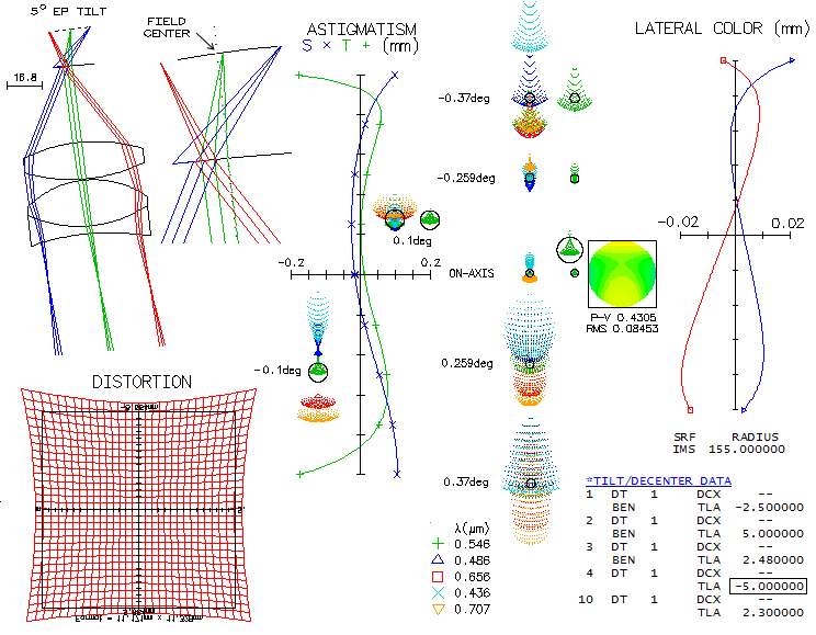
Field astigmatism can be better balanced by tilting eyepiece.
In most cases the needed eyepiece tilt is roughly
half of the image tilt, in the direction of image tilt. Raytrace
for 5° eyepiece tilt (below) shows
that to be the case, but at a
price of compromising some other image aspects.
Axial point is displaced from field center, with a better part of
the field radius - including center -
being astigmatic, in excess of the diffraction limited minimum
requirement (0.80 Strehl). The exit pupil
is in disarray, which likely generates additional eye aberrations.
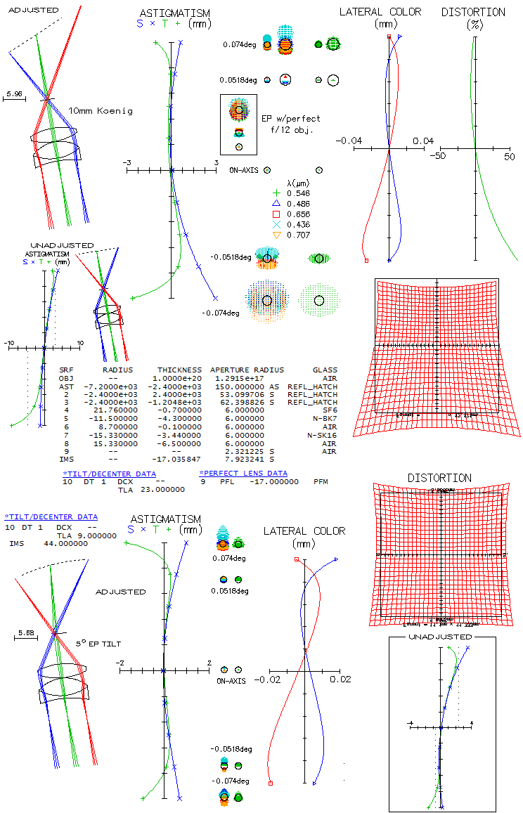
With a high-magnification eyepiece, like 10mm Koenig, and field
size somewhat smaller than the intended
by design, the image field is again very unbalanced astigmatism-wise
along the vertical field diameter,
with the only adjustment needed being in the tilt (top),
as much as 23°. Unadjusted - i.e. actual -
field has the top field
point displaced by about 3mm, and the bottom one nearly 5mm,
corresponding to over 10 and 16 diopters of
accommodation, respectively. Portion of the vertical field diameter
within 5 diopters is roughly 1/2 on
the top side, and somewhat more on the bottom (due to the shape of
astigmatic field). Lateral color is
somewhat assymmetrical, with the bottom vertical field radius
having the blue/violet remaining overcorrected
to the edge. Also, distortion
becomes extraordinarily high.
Both, astigmatism and distortion can be nearly balanced by tilting
eyepiece by about 5°.
Although some longitudinal astigmatism
is also induced to the central area (not noticeable due to its small
magnitude and small image scale),
it is insignificant, more so
due to the very small f-ratio of the beam focused by the eye
(i.e. "perfect lens"). Some lateral color
is induced to the axial point, but it is low enough to keep
all five wavelengths safely within the Airy
disc. Here, unadjusted field - i.e. field formed on the retina -
has the top point of the vertical field
radius displaced by about 2.3mm, and the bottom one by 0.8mm, i.e.
nearly 8 and 2.7 diopters, respectively.
It places the top area of the field out of average accommodation range,
but rest of the field is as shown
for the adjusted field at left.
As mentioned in the beginning, common wisdom with tilted elements
telescopes is to keep tilt angles as
small as possible in order to minimize aberrations and image tilt
(which itself becomes a source of
eyepiece aberrations). To illustrate how much it matters - or not -
with this particular system,
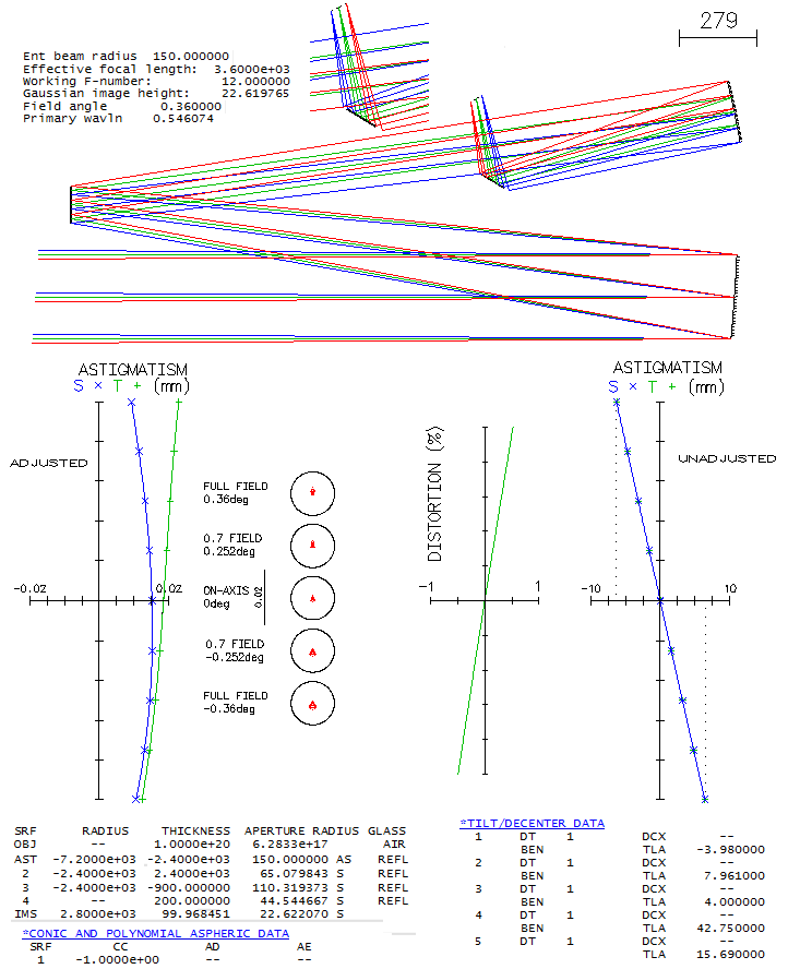
here is raytrace of a system with these same elements and separations,
only with tilt angles increased
so that a full 2-inch barrel eyepiece field can be accommodated.
Designing is simple: tertiary mirror is tilted
as much as necessary to place the flat outside of the light path,
and then the tilt of primary and secondary
is increased until the coma induced by tilting the tertiary is cancelled.
Adjusted field shows that despite significantly more of mirror tilt,
correction remains practically
perfect. However, image tilt increased to 15.69°, with the top
and bottom point of the vertical field
diameter displaced by 6.4mm, vs. 4.2mm with mirror tilt minimized.
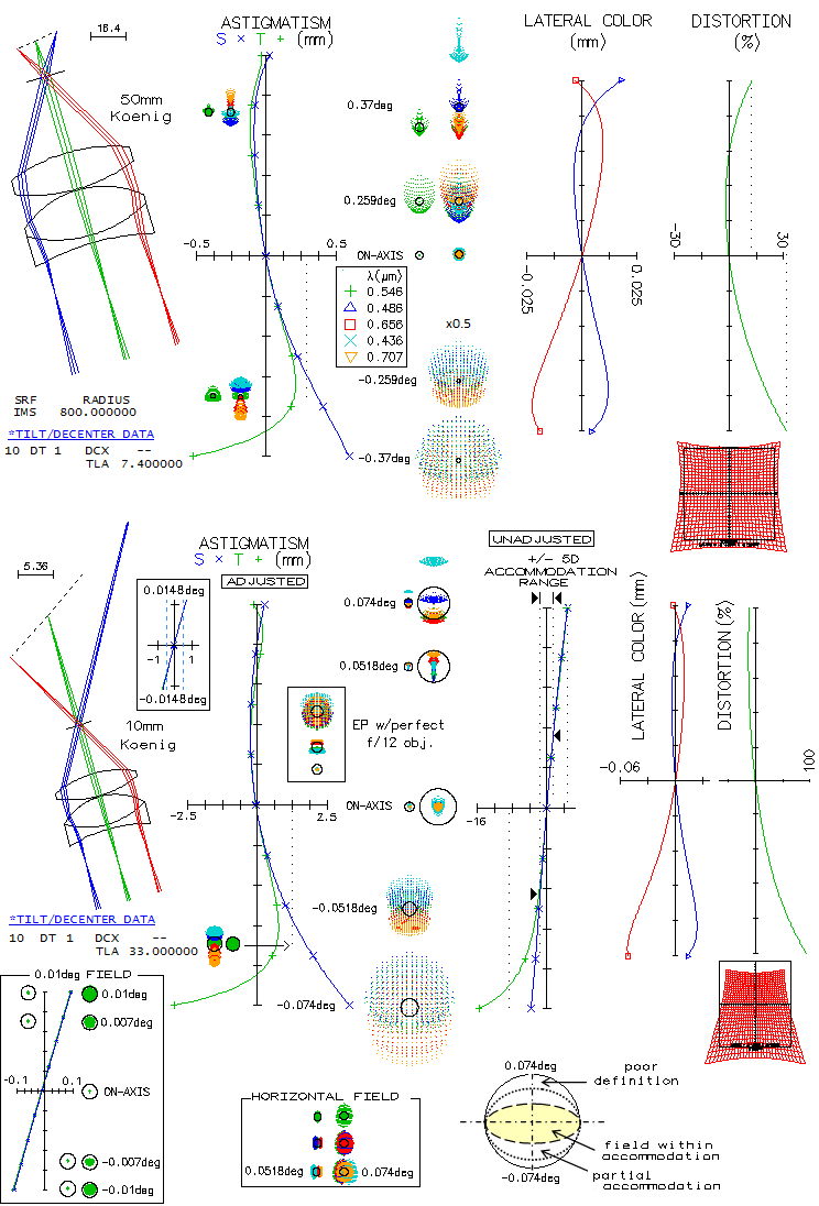
The effect of it on eyepiece image
is again evaluated using 50mm and 10mm f.l. units.
With the 50mm Koenig, the unadjusted field has top and bottom
vertical field diameter points displaced
by little over 1mm, or nearly 4 diopters. Since this is within
the accommodation ability of the average
eye, we can assume that the visual field will be about as corrected
as the adjusted field (7.4° image
tilt and 800mm field radius). The consequence of larger image tilt
is more of astigmatism imbalance along
the vertical field diameter: the top half is practically
astigmatism-free, while at the bottom point
it is nearly twice as large as with a perfect 300mm f/12 objective.
Lateral color error hasn't changed
significantly vs. smaller image tilt, but distortion is more out of
balance, and significantly larger
overall.
With the 10mm Koenig, adjusting to image tilt takes as much as 33°,
with an enormous distortion
imbalance. With unadjusted field, less than half of the vertical field
diameter is within +/- 5 diopters
accommodation range, with roughly half of the remaining field being
within some degree of partial
accommodation. Along the horizontal field diameter, correction is as
with a perfect 300mm f/12 objective,
with zero tilt. This confines useable field within an ellipse with
the top point at little less than 40%
of the top radius, bottom point at little over 40% of the bottom
radius, and a full field diameter
horizontally (the effect of tilting eyepiece is omitted, but it is
similar to that with the original
low-mirror-tilt system shown). Both, distortion and field
restriction are larger than with the
unadjusted 10mm Koenig and
the original system, but not dramatically so. It suggests that there
is little benefit from minimizing
mirror tilt with the Stevick-Paul design. While full 2-inch barrel
field may not be necessary, there is
no reason not to have full field for 1.25-inch
eyepiece barrel.
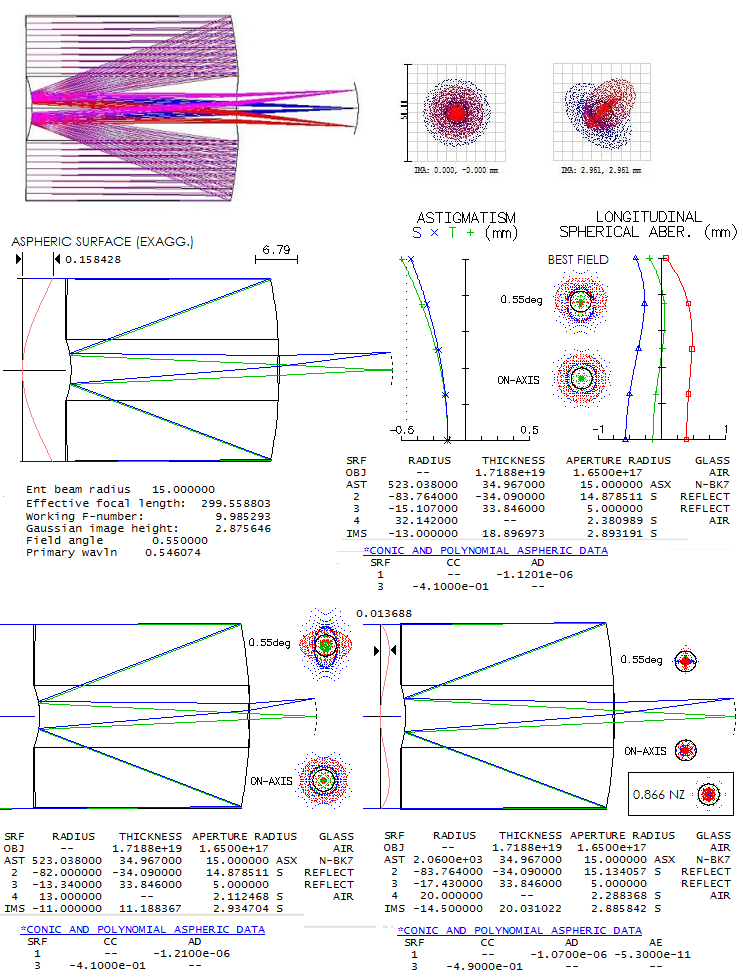
More than a decade ago, some details about this miniature SCT were
posted by its creator on an astro forum.
It aroused a great deal of curiosity and admiration. Functional
telescope made out of a single glass cylinder,
just large enough
to fit in the 1.25" eyepiece barrel. No prescription was published,
but the system layout, as well as ray spot
plots were posted (below, top). The spots reveal significant
longitudinal chromatism, lateral color error,
and relatively strong off axis astigmatism. The magnitude of
these aberrations is unexpectedly large for
such a small aperture, making uncertain whether raytraced system
was a design, or the actual system as it was
made.
Configuration nearly identical to the one posted achieves this
magnitude of longitudinal chromatism only with a
very strong curve placed on the aspherized corrector surface
(or, with the same effect, on the other side of the
corrector). There is no gain from having such a strong curve
neither with respect to fabrication, nor correction level.
However, lateral color error is roughly half of that in
the published spots, and astigmatism not noticeable (the original
off axis spots are given for corners of 4x4mm
field, hence they have a diagonal orientation). While the lateral
color error can be increased by weakening the
rear end radius, it would further diminish astigmatism.
On the other hand, achieving level of astigmatism
shown in the published ray spot plots would require significantly
stronger rear end radius, which would cause
configuration to significantly differ from the one posted (bottom left).
In other words, the ray spot plots
and layout published are not compatible. That indicates that the
ray spot plots and the system
layout posted may have come from two different systems.
If fully optimized, such system would use aspheric profile with
0.707 radius neutral zone, with the maximum depth
more than ten times smaller (13.7 vs. 158 microns, bottom right).
Posted description states 21 micron deep aspheric
curve, which is closer to one with 0.866 radius neutral zone (just
over 25 microns), but such profile would
produce significantly less of longitudinal chromatism (box above
last prescription bottom right).
Note that only the fully optimized system (0.707 NZ) uses 6th
order aspheric coefficient;
considering the magnitude of longitudinal chromatism,
the difference wouldn't be noticeable with the other two systems
(but is noticeable with the axial spot for
the 0.866 NZ system, which only has the 4th order coefficient).
In conclusion, posted
material was probably showing the first prototype of this amazing
little telescope, and some more or less related
raytracing material. If fully optimized, such system has impecable
correction of all aberrations, except the very
strong field curvature. Edge vs. center displacement is about 0.45mm,
which translates to 4.5 diopters of
accommodation (infinity to 0.22m) required with 10mm f.l. flat-field
eyepiece, over a field radius less than half
the field of view of a standard eyepiece of this focal length. Since
edge displacement is away from the eyepiece,
its pencil would exit it slightly converging, requiring unnatural
accommodation by relaxing eye lens beyond its
infinity mode. That would probably make it unachievable for
most people.
Harold A. Lower was amateur astronomer and astrophotographer based in
San Diego, CA. Back in the mid 1930s, not long after Bernhardt Schmidt
published his work, he and his son Charles built
an ultra fast 8-inch f/1 system of this type. It was the second
Schmidt camera built in the US -
back in 1932, a Riverside, CA dentist, Dr. H. Page Bailey built
an 8-inch f/2.8 Schmidt. But
the wide starry fields recorded with the Lower's camera got attention of
professional astronomers, and spurred construction and use of
large professional Schmidt telescopes in this country. In his
"Notes on The Construction of an f/1 Schmidt Camera", Harold
Lowers states that such camera can cover a 20° field, and be
"very useful for meteor photography and for the mapping of
areas of faint nebulosity".
His camera used a 12-inch f/1.33 (16-inch radius) pyrex
spherical mirror. Rough grinding took 98 hours and 25 pounds
of carborundum. After polishing the mirror, the usual way of
testing with a source slightly off axis produced astigmatism
making the mirror look warped. To overcome this, they had to
use unsilvered diagonal mirror to reflect the source - a
vertical slit - to the mirror, with the light reflecting back
through the diagonal to the tester's eye. Also, since it
was impossible to achieve uniform illumination over the
entire mirror surface, the knife-edge test was discarded
in favor of the Ronchi test, "which proved entirely
satisfactory".
As for the aspheric lens corrector, they decided to put aspheric
profile on one side, and to use "a combination of concave and
convex curves, as this type of lens would have less chromatic
aberration". This implies corrector with neutral zone either
at the 0.707 zone (the lowest wavefront error), or 0.866 zone
(the smallest ray spot plot). Since this strong corrector
is risky to make with the vacuum method, it was decided to
use subdiameter tools. Both, grinding and polishing tools were
made flexible, with a sponge rubber base and half-inch glass
squares cemented to the rubber with pitch (method first
employed by Bailey).
For the final testing, image of a bright slit placed in the
mirror infinity focus was observed from 20 feet, or more, distance
(as far as needed to have image of the slit project from top to
bottom of the mirror).
With spherical aberration corrected, light rays exit corrector
parallel, and image of the slit remains straight as the eye
moves toward beam edge; with sufficient spherical aberration,
image of the slit - a line of light - will curve (similar to
the Ronchi test). Lower does not specify sensitivity of this
test, only states it is sufficiently sensitive for a
photographic instrument.
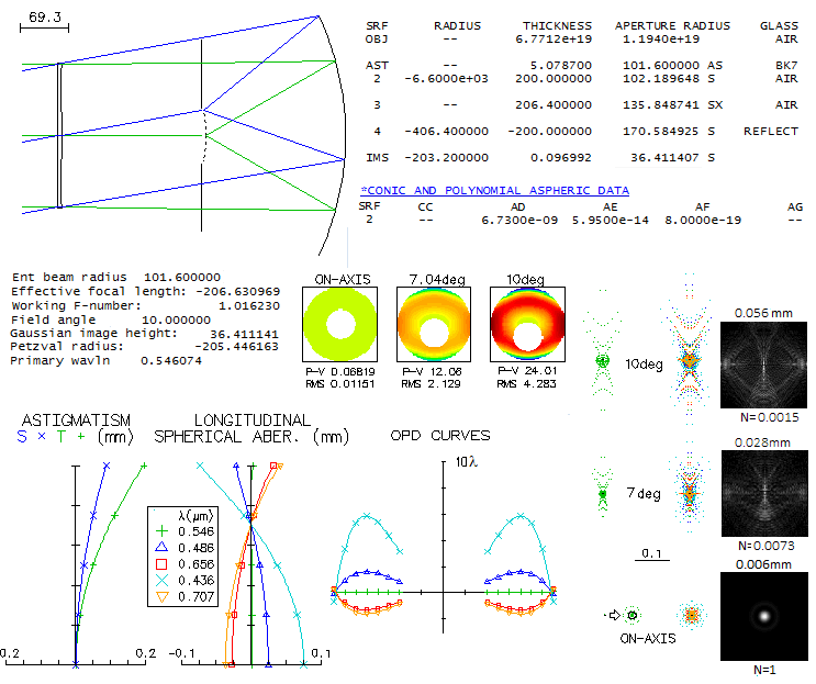
To illustrate what the imaging over 20-degree field with this
camera could look like,
below is a raytrace of near-perfect 8-inch f/1 Schmidt camera.
Central obstruction size wasn't specified by Lower; here, it is
put at 80mm in diameter, somewhat larger than
the 20-degree field. It blocks little more than 15% of light,
with the additional light loss close to the field edge, due
to the undersized mirror (it would take a 13.5 inch mirror to
fully cover the 20° field). This loss is near negligible,
adding only about 7% to that from the central obstruction
(for a little over 22% total).
While off axis aberrations in the outer field are crippling,
star images can be generally acceptable for film emulsions,
which form star images 10-30 microns in diameter, sometimes
larger. Diffraction images (even sensitivity for the five
wavelengths) 7° and 10° off axis
have very low normalization level (N), which means that they
are bloated spots of light, roughly 30 and 60 microns
in diameter, respectively, with a brighter extended vertical
core. This energy spread certainly significantly lowers the
camera's detection ability toward the outer field, both
magnitude and resolution-wise.
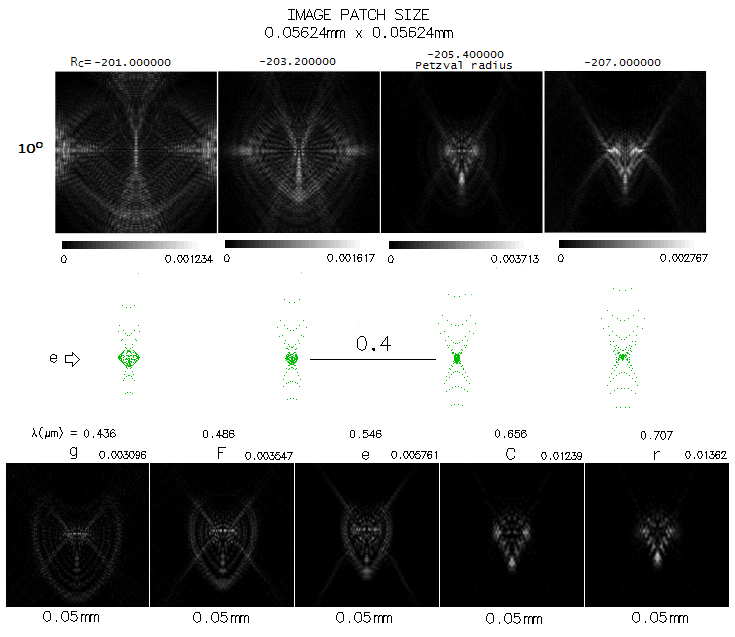
Looking at the 10° diffraction images for a few selected values
of image curvature (Rc) shows that the bright
portion of the image is the smallest for the curvature about
equal to the Petzval's (top below). Higher normalization values
selected by OSLO (below each image in the top row, and at the top
right corner in the bottom row), which are calibrated to produce
brightness of a certain level, also indicate that they are
inherently brighter.
However, polychromatic
encircled energy shows that it results in more encircled
energy only up to about 0.015mm radius, with the 80% energy radius
being about 50% larger than for R=-203.2mm (which could be indicated
by the ray spot plots' dense area size). Still, more compact
bright area should be advantageous resolution-wise. The image also
vary significantly with the wavelength, becoming smaller and more
compact toward the red (bottom; all images are of
the same scale, i.e. directly comparable size wise). These images
are 10° off axis on the Petzval curvature. The polychromatic
image for the Petzval curvature above shows that the red
wavelengths dominate, being smaller and with inherently
brighter core than the shorter wavelengths. Better correction
in the red is what certainly helped Lower to discover "Lowers
nebula" (Sh2-261), a faint 10th magnitude emission nebula
in the constelation of Orion (near its border with Gemini).
Its dominant spectral line is Hydrogen-alpha
(
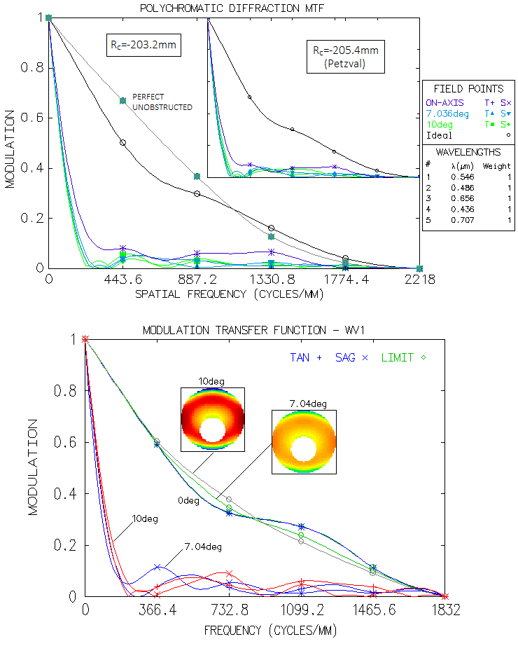
Taking it to the ultimate judge, the MTF, shows how devastating is
corrector chromatism at this fast focal ratio. Even on axis, contrast
transfer is roughly comparable to that of five times smaller
aperture (top below). It also dwarfs the advantage of smaller
diffraction spots along the Petzval surface. In the central wavelength,
contrast transfer is limited only by central obstruction (bottom graph).
Despite the smaller diffraction images, there is no obvious
advantage in contrast transfer at 7° vs. 10° off axis.
As a curiosity, as the central obstruction effectively shifts closer to
the edge, its effect diminishes, with the diffraction limit
coming closer to that set for a perfect clear aperture (not shown).
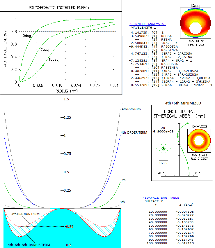
The best field curvature can't be determined by the P-V/RMS
values neither, since at this aberration magnitude they are very loosely
related to energy distribution and image shape. The usual
80% energy circle should give better idea of how wide is the
energy spread (below, top; note that it is given for the image
curvature in prescription, and is not necessarily the best
possible). It implies that the 10° image has smaller
energy spread vs. 7° image than indicated by their
respective image sizes, probably due to the brigther
central area.
Zernike coefficients for the 10° image (top right) show
as the most significant terms primary and secondary astigmatism
(#4 and #11, respectively), and primary spherical aberration (#8).
Off course, the actual aberrations are mainly lateral astigmatism and
oblique spherical aberration, but the program uses aberration
forms it's been supplied with. Similarly, best field does not
coincide with the best astigmatic field, since the latter shows
only primary and secondary astigmatism, and there are other
aberrations with astigmatism-like properties present (like the
two just mentioned, as well as elliptical coma, or arrows,
the basic form of trefoil, not balanced with tilt and coma).
Zernike term for primary spherical aberration
is whooping -7.13, implying 3.2 wave RMS of it, and on axis, the
actual spherical is nearly non-existent.
Below (left) is shown an exaggerated surface profile of the corrector.
The three power terms are given in their relative magnitude
one to another, as well as their sum with defocus (effectively
injected with the corrector radius term) needed to obtain a
profile with the same hight in the center as on the edge. The
two higher order terms are significant - particularly the 6th
order - and require significant additional deepening. This
profile - or at least close to it - is likely the one used
for the camera, since in his "Notes" H.A. Lower gives three
profiles, one for correction at paraxial focus, the second
for correction at marginal focus, and the third - the one
shown here - for correction at best focus location. Lewis
knew that the last one induces significantly less chromatism
than the other two.
It is all but certain that the actual camera was not as well
corrected as this exemplary system. Just omitting the smallest,
8th power term, induces several waves of spherical aberration,
which can be minimized by somewhat strengthening the 4th term
(bottom right, boxed).
With 2.5 waves P-V on axis, it is closer to the correction
level of the actual camera,
but it wouldn't make performance significantly worse. In fact,
it is not uncommon that the presence of spherical aberration
on axis results in better corrected outer field.
As the sag
table shows, this corrector is ~0.2mm deep at ~70% zone. One
wouldn't think it should be too hard to make one, but H.A.
Lower warned: it's a slow job.
Ludwig Schupmann's ingenious way of solving the problem of a
single lens chromatism has a small but dedicated crowd of
admirers among amateur telescope makers. A simple lens for the
objective, small concave mirror at its focus and a mangin mirror
corrector, about half the size of the objective, to make the final
image highly corrected - even over a relatively small field -
sound simple enough for obtaining medium aperture unobstructed
telescope practically free from chromatism. Those not deterred
by its relative bulkiness, and the need to tilt the elements,
put needed work into building one. Among them is Clif Ashcraft
from Perrinville NJ, who built a 7.25-inch Schupman and
described it on his
site.
Starting with the prescription given on the site, turned out
it is not the final system, rather the pre-design, made for a
final optimization with raytrace. It is a common step in
designing more complex system. The numbers are very close to
those that would be obtained following procedure described
on this site's Schupmann
page.
The initial system is f/13.3, with some residual spherical
aberration and longitudinal chromatism, that is best to take
care of at this stage, before goetting into tilting the elements.
Since that part is not included in the site description,
the actual Clif's system can't be exactly reconstructed, but
it will be interesting to see what needs to be done, and
what the final performance of cuch system is alike.
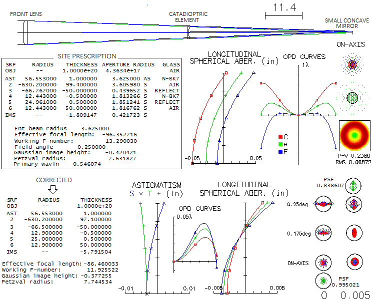
The top shows the optical scheme and the level of pre-design correction.
Spherical aberration is corrected by weakening the catadioptric element
(CE) front radius, and the resulting chromatism with a small change in
the separation and radius of curvature of the small concave mirror. As
a result, the system becomes f/11.9, and the final focus forms about
four inches before the mirror (hence the catadioptric element has less
than unit magnification). The astigmatic field is not flat, but the
curvature is mild: at 0.25° best focus is 0.127mm off of the
central point plane, requiring only ~1.3 diopters of accommodation
with 10mm f.l. eyepiece (corresponding image radius of curvature is
~22 inch, convex toward the CE).
The real fun starts now. To make the final image accessible,
it is necessary to tilt the small mirror, in order to get the CE out
of the converging cone from the objective, and then tilt the CE in
order to take the final image out of that same cone, to a location
convenient for observing (that includes use of a small diagonal mirror
near the final image). Tilt angles are not specified, but the
illustrations on the page show that they are about the smallest
possibe, in order to keep tilt aberrations low, at a price
of having quite restricted usable field without the CE or
diagonal mirror intruding into the light path (altough, arguable,
small intrusions into abaxial beams, having in fact negligible
effect, would be a good trade off for keeping tilt aberrations
at their minimum).
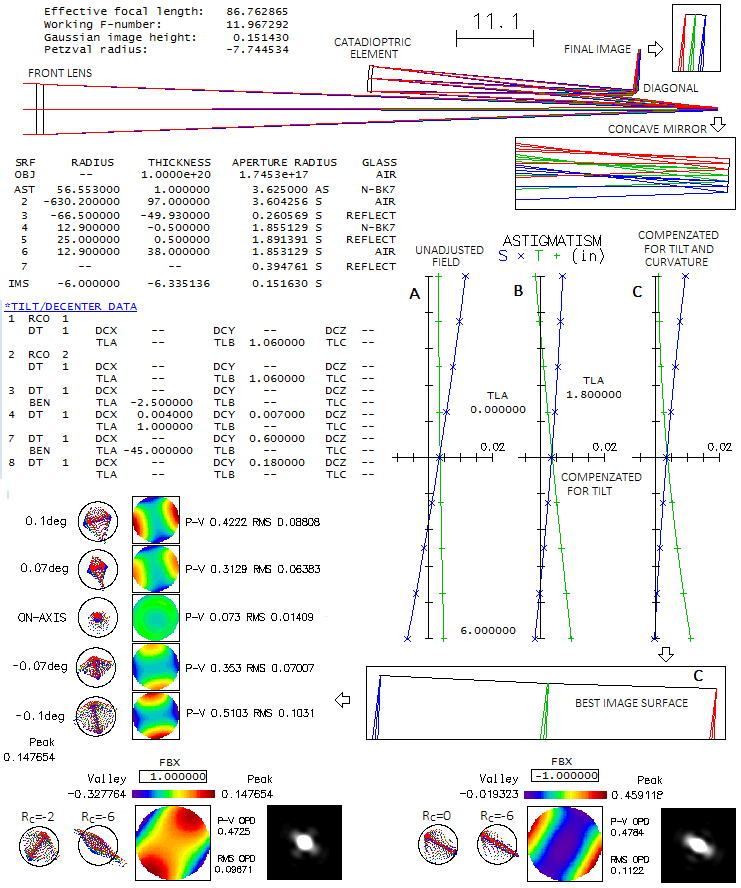
Optical scheme of the Schupmann with the first three elements tilted, and
a diagonal added to reflect the final image away from the mirror (top),
is how it is commonly done. The most significant aberrations included
by tilting is astigmatism, followed by much generally low in comparison
lateral color and a trace of coma. Nearly all astigmatism originates
at the CE, tilted one degree around its horizontal axis. In order to
offset this astigmatism, the front lens is tilted slightly over 1 degree
around its vertical axis. Lateral color, affecting entire image, is
minimized by a slight decentering of the CE in the right dirrection.
Here, all corrections are done by adjusting the elements' separation,
or centering; it could be done by adjusting the radii, but it is
considerably more involved in practce, and probably wouldn't produce
significantly better results.
In order to acces correction level over the best image field,
the astigmatic field needed to be tilted by 1.8°, and some
field curvature needs to be included. Visually, it is of little
consequence, since the image over this small field is well
within accommodation ability of the eye (however, extending
field to the maximum fitting the 1.25" eyepiece barrel would
be challenging in this respect). The two field sides along the
vertical field diameter are not strictly symmetrical, but the
difference is quite small. Along the horizontal field diameter
(bottom), the optimum tilt/curvature parameters are different,
but the unadjusted diffraction images at 0.1° (shown) are
not very different from those brought to the best focus
(again, this is likely to be significantly more pronounced with
wider fields). The final image is, in fact, double tilted:
tilt of its Y-axis (contained in the same plane with system's optical
axis) comes from the tited CE, and image tilt along X-axis,
perpendicular to it, from the front lens tilt. However, both
are generally small, with little effect.
The tolerances for the lens-to-mirror and mirror-to-CE separation are
not too rigid; for the former, axial deviation of 1/10 of an inch,
or somewhat more, is negligible, and for the latter about half as much
(both affect primarily longitudinal chromatism). However, decentering
the mirror or, more so, the CE, by even a fraction of 1/10 inch,
will cause noticeable lateral color error across the image field.
The shortening of the focus due to the correction of the front CE
radius can be, if desired, reversed simply by changing the separation
between the lens and mirror, and between mirror and CE. Here,
in order to extend the
final focus so that the CE-to-focus separation nearly equals that of
the mirror-to-CE separation, the mirror-to-CE separation is reduced
to -49, and lens-to-mirror-separation to 95 (mainly to correct
longitudinal chromatism).
This changes the focal ratio to f/12.6, and causes no appreciable change
in the overall correction. Since the final focal ratio according to
Clif's site is f/14, he probably decided to extend the final focus somewhat
beyond the small mirror. That makes possible either to decrease tilts of
the CE and front lens, lowering field aberrations, or use of wider fields
with given tilts (the elements here, and on Clif's side are tightly
packed together, limiting field size to not much larger than 0.1°).
◄
14.1. Early telescopes
▐
14.3. Observatory telescopes
►
|