|
telescopeѲptics.net
▪
▪
▪
▪
▪▪▪▪
▪
▪
▪
▪
▪
▪
▪
▪
▪ CONTENTS
◄
6.5. Strehl ratio
▐
6.6.1. MTF - aberration compounding, CCD, limitations
► 6.6. MTF - Modulation transfer function
PAGE HIGHLIGHTS Modulation transfer function (MTF) is commonly used to describe the convolution of point spread functions (PSF) and the Gaussian (geometric) image of an object that is a continuous sinusoidal intensity pattern, in effect a continuum of dark and bright lines gradually changing from the maxima (in the middle of the bright line) to minima (middle of the dark line). The convolution integral sums up energy arising from the PSF blotches created at every point of the Gaussian image, and so describes the corresponding diffraction image of the pattern. Changes in the PSF due to aberrations, pupil obstructions and other factors affect the quality of this diffraction image, specifically its contrast level and phase distribution. In general, convolution with the PSF smoothes out, i.e. flattens intensity distribution of the sinusoidal (or any other) pattern, lowering the contrast and acting as a low-pass filter (i.e. imposing limit to resolution) - the larger PSF vs. pattern's frequency, the more so. The MTF is a part of the complex function describing this process, called Optical transfer function (OTF). While OTF is limited to the effect of system PSF on imaging this single form of object - a sinusoidal intensity distribution - it is accepted as a performance indicator for imaging in general. The OTF consists of two components: (1) MTF, and (2) phase-transfer function (PTF). The former is its modulus, or magnitude, expressing the relative change in contrast of the pattern image vs. aberration-free aperture, and the latter quantifies the linear lateral shift of this pattern caused by the change in PSF intensity distribution due to aberration. That intensity distribution change may be radially symmetric (such as draining of the energy from the central maxima with defocus or spherical aberration), or asymmetric, for example due to coma aberration (FIG. 100, middle). The basic relation between OTF, MTF and PTF can be presented as:
OTF = |OTF|e iPTF
= MTFe iPTF
implying that the MTF is the absolute value of the OTF (e
is the natural logarithm base, 2.718; note that the equality is not
present with the commonly used form of the OTF, MTF, which entirely omits the phase factor). Since OTF contains
the imaginary
number i, it is a complex function consisting from the
real and imaginary part, the latter being the part containing the imaginary
number. The imaginary number i=(-1)0.5
is convenient for expressing angular shifts, in this case angular shift of
the sinusoidal MTF intensity pattern phase at a given Gaussian image
point due to the pattern's lateral shift, caused by aberrated PSF. With
eiPTF=cos(PTF)+isin(PTF),
the two parts of OTF function can be expressed as:
OTF = MTF[cos(PTF) + isin(PTF)] = MTFcos(PTF) + MTFisin(PTF),
with the two factors at right being the real and imaginary part of the OTF, respectively (noting that the PSF
is usually annotated as angle). Either can be plotted separately, the
former, being cosine function, originating at 1 for zero spatial
frequency, and the latter originating at zero. If PSF retains any form
of symmetry around a line splitting it in two halves (i.e. symmetry in
its pupil aberration function), the imaginary part vanishes (because in
such case the shift can only be zero or π,
for contrast reversal), and OTF reduces to OTF= MTFcos(PTF).
This is the case with defocus, spherical aberration and astigmatism, for
any orientation of the PSF, and with coma only for a single orientation,
along the axis of aberration. For all other orientations the coma OTF
consists of both, real and imaginary part.
It is important to note that, since eiPTF=cos(PTF)+isin(PTF)
does not represent a sum, rather coordinates of a complex number, the
real part of the OTF does not represent the magnitude of OTF (i.e. MTF),
except when PTF equals zero (no phase shift). If we use the common
notation for the real and imaginary part, Re and Im,
respectively, then the relation between them and the MTF is given by |OTF|= MTF= (Re2+Im2)0.5.
As illustrated below, eiPTF
is not a value, rather phase descriptor. Hence OTF magnitude is not
affected by it.
OTF can also be defined in terms of PSF, as OTF
Or, more directly, just as the
Fourier transform of aberration-free pupil
function
(i.e. Fourier transform of the square pulse) is sinc function, so is the
Fourier transform of triangular function
- which is the form of aberration-free 1-D OTF for square
pupil, with the OTF form for circular pupil being only slightly
different - the sinc
function squared, or PSF. In other words, the PSF is proportional in
form to the continuous spectrum of frequencies contained as a sum of
harmonics in the triangular (or near-triangular) function form.
It is important to note that the OTF relations above are, by their basic concept, valid only for incoherent light. Formal
derivation states that this type of pattern in coherent light would be
reproduced without any distortions in amplitude or phase, i.e. with 100%
contrast transfer, with the sudden drop to zero at the cutoff frequency
2λ/D (coherent transfer
function).
As above relations show, MTF does not
include possible lateral shift of intensity pattern in any way. This is
not by choice, rather by the inherent property of MTF defined as the
modulus (magnitude) of contrast transfer as a function of spatial frequency, with
every spatial frequency treated as an isolated contributor to the
function. Thus, lateral shift of the pattern is no factor, only the
contrast level is recorded. MTF alone shows the efficiency of contrast transfer
from the object to
its image with zero intensity phase shift, for a single orientation in the aberrated image, normally that
along the axis of
aberration. However, 180° (π
radians) phase shift, which can be caused by large amounts of
aberrations, will result in contrast reversal, i.e. switch of
bright and dark areas in the image vs. object. For instance, such image
of F, in addition to it being distorted by the large level
of aberration, could make it unrecognizable, even if contrast needed for
detection is there. Hence, the OTF phase factor is potentially important
factor in predicting image quality, but only in the presence of large
aberrations, well above the level found near axis in optical telescopes
(for instance, contrast reversal due to primary spherical occurs at near
2λ
P-V wavefront error).
Similar to MTF is the contrast transfer function (CTF),
the difference being that the latter describes impulse response (i.e.
contrast change in the image vs. object) based on an object that is a
continuous square wave intensity distribution, in effect a continuum of
bright and dark lines with even intensity distribution over
them.
Some additional basic aspects of the OTF/MTF
are given below. INSET A illustrates characteristic form of the MTF,
showing contrast drop as a function of spatial frequency
ν
for brightly illuminated object with high inherent contrast, as well as
the effects of change in illumination/contrast level. For
comparison, graph also shows the CTF. INSET B illustrates the
effect of phase shift, INSET C shows OTF expanded to include
radial PSF dimension and its effect, and INSET D illustrates
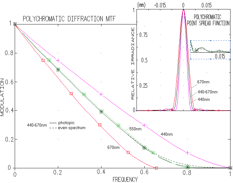
polychromatic MTF.
INSET A:
TOP LEFT: Standardized MTF object form
is a continuum of parallel, equally spaced
bright contrasty lines on dark background, with irradiance
modulation defined as infinite sinusoidal distribution. The line width, equaling that
of the dark/light pair, is
inversely proportional to the spatial frequency
ν,
normalized to 1 at the cutoff frequency D/λ cycles per radian (the
inverse of the angular limit to resolution λ/D
in radians, D being the aperture diameter), where image
contrast drops to zero (linear cutoff
frequency is the inverse of the linear limit to resolution
λF,
or 1/λF in lines per mm, for λ in mm). This form of
intensity distribution can be represented as periodic sinusoidal wave,
with the contrast determined by the relative intensity of its maxima
vs. minima. Image of this pattern has the relative intensity and
contrast dampened due to the effect of
diffraction, whether without
or with aberrations present, At any given frequency, MTF is a
ratio of the output (image) to input (object) modulation amplitude.
Mathematically, it is Fourier transform of the system's
PSF (more specifically, it is
an integrated sum of the PSFs for every point over its intensity
distribution profile, i.e. convolution of object's Gaussian image
and aperture's PSF). At
the limit of resolution for aberration-free aperture, the line width
is nearly equal to the aperture's
FWHM.
At right, shown is the effect of 1 wave P-V of
defocus on the image of an object that is not the standard MTF
pattern, but one in which bar width is oriented horizontally, with
the line width changing continuously according to the spatial
frequency. Top image (A) is aberration-free, and bottom (B)
defocused one. If the aberration is large enough - in the case of
defocus ~0.9 wave P-V or larger - image of such object will show
contrast reversal - where bright lines become dark and vice versa - indicated by the OTF, but not the MTF. The reason
was immediately apparent from the PSF intensity distribution for 1
wave of defocus, developing dark circle (minima) at the center of
the pattern. Hence, MTF does provide information on contrast
transfer, but not on the image itself. To reconstruct the image, we
need OTF. This, however. may have significance only with large
aberrations, generally about 1 wave P-V and larger (a few more
examples at ). OTF for smaller aberrations does not fall below zero,
thus there is no contrast reversal to affect image.
For aberration-free clear aperture, the MTF
is given by MTF=(2/π)[cos-1ν-ν(1-ν2)0.5].
It can be also expressed as:
with the angle α
in degrees found from cos(α)=ν
(for software use, the angle obtained from arccos(ν) is in radians,
hence needs to be multiplied with 180/π for degrees; the
corresponding form for the first factor is then 2arccoss(ν)/π).
Graphically, MTF
contrast transfer equals the relative overlapping area of two
identical circles, in units of the circle area (FIG. 62, top
right), with the circle diameter normalized to 1, and the center
separation s=ν
varying from 0 when the circles are coinciding (ν=0),
to 1 when only touching (cutoff frequency ν=1).
Similarly, the normalized MTF for
reduced aperture (still of
unit diameter, with v=0 when the two circles are touching, smaller
inside the larger), equals the overlapping area with the smaller
circle appropriately reduced in diameter, with overlapping area
being in units of the smaller circle area. The actual range of
resolvable frequencies of a smaller aperture is in proportion to the
aperture reduction factor. In terms of MTF, CTF is given as
CTF=(4/π)[MTF
Graph below illustrates normalized frequency implications with
respect to MTF pattern characteristics. Since cutoff frequency
is given in frequency form, as D/λ, the inverse of the actual
resolution, the
lower frequency, the wider pattern. With the resolution at cutoff frequency,
λ/D, being 2.44 times smaller than the angular Airy disc
diameter (given by 2.44λF/f, f being the focal length,
hence equaling 2.44λ/D), the pattern width is proportional
to the inverse of normalized frequency: it is twice wider than at
the cutoff at 0.5 frequency, five times at 0.2 frequency, and so on.
To express it in Airy disc diameters, it only needs to be divided
by 2.44 (so it will be 2/2.44=0.82 Airy disc diameters wide at 0.5
frequency).
It is important to understand that the MTF
graph, such as the one above, does not set absolute values for
the contrast drop, or limit to resolution. Both are strictly applicable only
to the particular MTF object form used for its calculation: a sinusoidal pattern of
bright lines on dark background, λF/2ν
wide linearly, F being the focal ratio f/D (i.e. linear width of
the bright line at resolution limit is
λF/2, or nearly one fifth of Airy
disc diameter). Actual contrast
drop-off and limiting resolution will vary with the specific properties
of details observed, background, and peculiarities of eye perception, or
detector properties. For non-continuous patterns, sinusoidal,
square-wave, or others, contrast transfer will generally increase with
the reduction in the number of lines (FIG.
103).
One example is
the resolution threshold for low-contrast MTF-like planetary details which is,
according to the LCB threshold level in FIG. 100, approximately half
of that for
brightly illuminated contrasty object. Another is a dark line on light
background, which can be detected at an angular width several times smaller
than the angular diffraction resolution limit
for point-images of ~λ/D radians, because it is the
Edge Spread Function,
not the PSF, that is applicable in determining its diffraction intensity
distribution.
An actual object that
comes very close to the standardized MTF scenario is a pair of nearly
equally bright stars at the optimum brightness level. Resolution-wise,
the MTF limiting resolution (cutoff frequency) is nearly identical to the empirical Dawes' limit in double star
observing. However, for pairs farther from the optimum brightness level,
or,
especially, pairs with significant difference in brightness, the resolution
limit is lower, or much lower.
Still, despite the MTF being
standardized to a single object form sample and brightness level, it is considered to be a reliable
general indicator of the effect of wavefront aberrations - or any other
factor affecting wave interference in the focal zone - on image quality.
As mentioned, given relatively low RMS wavefront level of any aberration will result in
near-identical overall contrast loss, but
the specifics will vary somewhat. FIG. 101 illustrates variations in
the aberrated PSF
(left) and MTF (right) for common wavefront aberrations of 1/13.4 and
1/6.7 wave RMS (graphs generated by Aberrator
freeware, Cor Berrevoets).
FIGURE 101: PSF and MTF plots for clear aberration-free aperture
(black), and aberrated (red) at the 0.80 Strehl level, and that
wavefront error doubled.
DEFOCUS: 1/4 and 1/2 wave P-V. Doubling the error halves the peak
PSF intensity (Strehl), but the average contrast loss is three times
greater (20% vs. 60%, given as a ratio number by the differential
between the Strehl and 1). Note that the Strehl for 1/4 wave WFE of
defocus is slightly higher than 0.80.
PRIMARY SPHERICAL ABERRATION: 1/4 wave and 1/2 wave P-V errors have
nearly identical effect on the PSF maximum as with defocus, but the
more widely spread energy causes more of contrast loss at the lower
frequencies, while the smaller central maxima results in somewhat
better transfer at mid-to-high frequencies. The transfer is again
inferior near the cutoff due to the smaller bright core with
defocus. Being close to zero, the cutoff frequency for 1/2 wave P-V
is about 20% lower in field conditions.
PRIMARY ASTIGMATISM: The effect of 0.37 and 0.74
wave P-V is similar to 1/4 and 1/2 wave of defocus in that the
energy spread out of the Airy disc is mostly contained closer to
central maxima, resulting in less of contrast loss at low
frequencies. Unlike defocus, does not change radial symmetry of PSF,
astigmatism gives to it cross-like shape which, similarly to coma's
asymmetry, gives the best contrast transfer when cross orientation
is identical to that of the bars (green) and the worst when it is at
45° angle.
TURNED EDGE: 2.5 waves P-V is needed that turned
edge starting at 95% the radius to lower the Strehl to 0.80. Lost
energy is evenly spread wide out (the abrupt initial contrast loss
ending at about 1/40 frequency indicates the radius of this spread
as 40 times the cutoff frequency, or 40λF - over 30 times the Airy
disc radius). Odd but expected TE property - due to the relatively
small affected area (the RMS for 0.80 Strehl is whooping 0.28 wave)
- is that increasing the aberration does almost no additional
damage.
ROUGHNESS: ~1/14 and ~1/7 wave RMS of roughness
producing asymmetric PSF pattern, thus having contrast transfer vary
with its orientation relative to MTF bars. Due to the random nature
of the aberration, the P-V wavefront error can vary significantly
for any given RMS/Strehl level. IHere, the P-V error ranges from
-0.169 (blue speck on the wavefront map) to 0.374, and -345 to
0.745, respectively. RMS error also may not be as reliably related
to the Strehl as with most other aberrations.
PINCHING: 0.37 and 0.74 wave P-V of wavefront
deformation caused by edge pinching at a three 120°
separated points has the typical
SEEING ERROR: Averaged PSF/MTF effect of ~1/14
and ~1/7 wave RMS of atmospheric turbulence. The P-V error can vary
substantially (here is 0.43 and 0.86 wave, respectively). Seeing
error fluctuates constantly around the average, as do the
corresponding image contrast and resolution. Larger seeing errors
(1/7 wave RMS is rather common with medium size apertures) reduces
contrast level to that similar to twice smaller aperture for
low-to-mid frequencies, with some high-frequency transfer (iincluding limiting
resolution) advantage remaining.
MTF contrast transfer generalized to the RMS
wavefront error alone, regardless of the type of aberration is, as
shown by Bob Shannon, given by a product of aberration-free MTF and the Aberration Transfer
Function [ATF=1-(ω/0.18)2(1-4(ν-0.5)2),
where ω is the RMS wavefront error in units of
wavelength, and v is the
normalized spatial frequency; not to confuse with the
Amplitude Transfer Function - this
is the only place where the Aberration Transfer Function is mentioned] for any given level of the RMS error,
and aberration-free
|
||||||||||||||||||||||||||||||||||||


 INSET
C: In addition to phase shift,
if PSF intensity is varying radially it will also cause different contrast transfer for different
orientations of the PSF relative to MTF pattern. A complete MTF integral has
radial component, thus it integrates for all orientations of the PSF
relative to the line pattern. Graphically, it is
represented by a volume figure, formed by continuous change of the
integration angle (i.e. pattern orientation) through a full circle,
or 2π radians
(right). This volume may be looked at as a total contrast, transfer.
INSET
C: In addition to phase shift,
if PSF intensity is varying radially it will also cause different contrast transfer for different
orientations of the PSF relative to MTF pattern. A complete MTF integral has
radial component, thus it integrates for all orientations of the PSF
relative to the line pattern. Graphically, it is
represented by a volume figure, formed by continuous change of the
integration angle (i.e. pattern orientation) through a full circle,
or 2π radians
(right). This volume may be looked at as a total contrast, transfer.


 MTF, as illustrated at left
for selected levels of RMS wavefront error (ω). It clearly
shows that contrast transfer does not drop linearly, but
exponentially with the increase in the RMS error. While the contrast
loss is still negligible for ω=0.037 (1/8 wave P-V of primary
spherical level), it is several times larger at the error doubled.
Another 50% higher error, to 0.10 wave RMS, nearly doubles the loss,
but yet another 50% increase, to 0.149, more than doubles the entire
contrast loss at ω=0.10.
MTF, as illustrated at left
for selected levels of RMS wavefront error (ω). It clearly
shows that contrast transfer does not drop linearly, but
exponentially with the increase in the RMS error. While the contrast
loss is still negligible for ω=0.037 (1/8 wave P-V of primary
spherical level), it is several times larger at the error doubled.
Another 50% higher error, to 0.10 wave RMS, nearly doubles the loss,
but yet another 50% increase, to 0.149, more than doubles the entire
contrast loss at ω=0.10.